I took a pistol course in undergrad, and while I was a poor marksman I enjoyed the experience. In particular, I was surprised by how meditative the act of shooting was. As our instructor explained, much of good shooting comes down to not doing anything when you pull the trigger. When you’re not firing, it’s easy to point a gun at a target and line up the sights, but as you pull the trigger you subconsciously anticipate the noise and movement of the pistol blast, which makes you flinch and pull the gun off-target. Being a good shooter thus requires consciously learning to counteract what your instincts tell you to do.
If you believe Bill Carr and Colin Bryar’s book on Amazon, Working Backwards, Amazon’s success can be understood in similar terms. According to Carr and Bryar, Amazon alone among the West Coast zaibatsu has succeeded not because of some big technical or social insight (Google Search, Windows) but because of a long series of canny business decisions. Bezos has said something similar: “Amazon doesn't have one big advantage, so we have to braid a rope out of many small advantages.” The implication is that you too can build an Amazon-quality firm; you don’t need any flashes of mad genius, just the ability to eke out small advantages through savvy management.
(This might seem like an insane claim, but it’s worth noting that Amazon has indeed launched a ton of successful and loosely coupled businesses: in addition to their core commerce business, there’s AWS, Amazon Robotics, Kindle, Prime Video, Fire TV, and a bunch of other stuff. Contrast this to Google’s recent track record…)
What’s more, Carr and Bryar go on to argue that Amazon’s business acumen is driven not by some inscrutable Bezos magic but by adherence to a simple set of principles. And these principles aren’t esoteric or Amazon-specific—almost any business can follow them. The reason so few businesses have copied Amazon’s success is simply because each principle defies human nature in some way. Just like pistol shooting requires one to unlearn one’s instincts and pull the trigger without moving any other muscles, being an “Amazonian” business requires discarding what you think you understand about building a business and going back to basics.
So, what are these magic principles?
1. Focus on Customers, Not Competitors
Focusing on competitors is human nature—in a competition, we judge ourselves based on our rivals, and like to imagine how we’ll defeat them. But success in business comes from satisfied customers, not vanquished foes, and keeping a relentless focus on users/customers is key to building something great. This is hardly Amazon-specific wisdom: “build something people want” is venerable YC advice, and Zero to One also makes the point that competition is bad and focusing on it counterproductive. Perhaps the fact that so many different people feel the need to emphasize this point speaks to how counterintuitive it is: were it widely adopted, it wouldn’t be repeated.
Plenty of people outside business also get this wrong. A few weeks ago, a friend was explaining how he feels that many computational chemists are making software not for users but for other computational chemists. This is a case in which writing papers leads to different incentives than releasing products: papers are reviewed by one’s peers (other computational chemists), while products are ultimately reviewed by users. Hopefully Rowan doesn’t make this mistake…
2. “Bar Raisers”: External Vetos in Hiring
Amazon includes a person called a “Bar Raiser” involved in all hiring decisions, who isn’t the hiring manager (the person who is trying to acquire a new team member) but who has final veto power on any potential hire. The hiring manager is hiring because they need help in the short term, so they’re typically willing to engage in wishful thinking and lower their standards—but the Bar Raiser (who’s just another Amazon employee, with a bit of extra training) has no such incentives and can make sure that no poor performers are hired, which is better for Amazon in the long run.
I like this idea because it’s a nice example of mechanism design: just a little bit of internal red-teaming which (according to the book) works quite well. (Red teaming is another one of those “good but counterintuitive practices” which seems underutilized—see the discussion in a recent Statecraft interview.)
3. Problem-Focused, Not Skills-Focused
It’s natural to think about what we should do next in terms of what we’re good at: “I’m good at X, how can I use X to solve a problem?” Carr and Bryar argue that “working forwards” in this way is stupid, because only at the end do you think about who (if anyone) might care if you succeed. “Working backwards” from problem to solution is a much better strategy: first you articulate what you might need to accomplish to produce a compelling solution, and then you think about if you can do it. Inside Amazon, most potential new projects start out by drafting what the press release might be if the project were finished, and then working backwards from the press release to what the product must be. (Most products envisioned in this way never actually get developed, which is exactly the point of the exercise.)
George Whitesides has advocated for a similar way to approach science: first write the paper, then conduct the experiments. Lots of scientists I know find this repulsive, or contrary to how science should be practiced, but it always seemed shrewd to me—if you can’t make an interesting paper out of what you’re doing, why are you doing it? (Exploratory work can be tough to outline in this way, but there should be several potential papers in such cases, not none.)
4. Single-Threaded Leadership
As organizations scale, it becomes tougher and tougher to allow teams to work autonomously, and responsibility and authority for almost all projects ends up bestowed upon the same small number of people. This makes insightful innovation hard: to quote Amazon SVP of Devices Dave Limp, “the best way to fail at inventing something is by making it somebody’s part-time job.” Amazon’s solution is the idea of single-threaded leadership (STL, probably someone’s idea of C++ humor). Organizations need to be arranged such that individual teams can respond to their problems intelligently and independently, planning and shipping features on their own, and each team needs to have a “single-threaded leader” solely responsible for leading that team.
Instituting STL takes a good amount of initial planning, since dividing up a giant monolith into loosely coupled components is tough both for software and for humans, and it’s not in the nature of authorities to relinquish control. If done properly, though, this allows innovation to happen much faster than if every decision is bottlenecked by reliance on the C-suite. (It’s sorta like federalism for businesses.)
This idea matters for labs, too: some research groups rely on their PI for scientific direction in every project, while others devolve a lot of authority to individual students. The latter seem more productive to me.
5. Bias Towards Action
Humans are by nature conservative, and sins of commission frequently feel worse than sins of omission—making a bad decision can cost you your job, while not making a good decision often goes unnoticed (the “invisible graveyard”). To counteract this, Amazon expects leaders to display a “Bias for Action.” In their words:
Speed matters in business. Many decisions and actions are reversible and do not need extensive study. We value calculated risk-taking.
Again, this echoes classic startup advice: “launch now,” “do things that don’t scale,” &c.
6. No Powerpoint!
In June 2004, Amazon banned PowerPoint presentations from meetings, instead expecting presenters to compose six-page documents which the entire team would read, silently, at the beginning of each meeting. Why? A few reasons:
PowerPoint lends itself poorly to complex or nuanced ideas, whereas written documents can contain more information and more complete chains of reasoning.
PowerPoint leads to “slick,” well-rehearsed presentations where the presenter’s style and charisma matters as much as the underlying ideas.
Writing enforces greater clarity of thought than speaking.
PowerPoint makes the audience passive, while reading makes the audience active participants in the ideas. People like to be passive, and it’s fun to hear an inspiring presentation, but in the long run it’s better for everyone to actually engage.
I’m pretty sympathetic to these criticisms. Most high-stakes academic events today revolve around oral presentations, not papers—although papers still matter, doctorates, job offers, and tenure are awarded largely on the merits of hour-long talks (e.g.). As a result, I spent a ridiculous amount of my PhD just refining and hearing feedback on my presentations, much of which had nothing to do with the underlying scientific ideas. Perhaps this focus on showmanship over substance explains why so little science today seems genuinely transformational. (It’s also worth noting that presenting, much more so than writing, favors charismatic Americans over the meek or foreign.)
There are, of course, more than just these six ideas in Working Backwards, but I think this gives a pretty good sense of what the book is like. Overall, I’d recommend this book: it was interesting throughout (unlike most business-y books), and even if nothing in its covers is truly new under the sun, the ideas inside are good enough to be worth reviewing periodically.
“Like arrows in the hand of a warrior are the children of one's youth.”
–Psalm 127:4
Mata Mua, by Paul Gaugain (1892), another Westerner looking for enlightenment among “venerable cultures.”
What if our most fundamental assumptions about parenting were wrong? That’s the question that Michaeleen Doucleff’s 2021 book Hunt, Gather, Parent tries to tackle. Hunt, Gather, Parent (henceforth HGP) documents Doucleff’s journey to “three of the world’s most venerable cultures”—the Maya, the Inuit, and the Hadzabe (in Tanzania)—to learn about how they parent their children, and offers helpful advice for parents envious of the kind, helpful, and responsible children she observes.
Doucleff’s writing hits some familiar beats: critiques of helicopter parenting, distrust of endless after-school activities, and laments about the atomization of our society (cf.). But there are plenty of unexpected insights too. I was convicted by her account of how Hadzabe children are given autonomy and responsibilities from a young age without being either ignored or micromanaged: her vision of a middle ground between K-selected “helicopter parents” and r-selected “free-range parents” was compelling.
There’s a lot to like about the parenting depicted in HGP. For instance, Doucleff highlights how toddlers’ innate eagerness to help is used by the Maya to build a culture of helpfulness (the virtue she calls acomedido) which lasts as they grow, whereas American parents generally disregard help from a toddler and thus teach kids that their help isn’t valued. On the other hand, I’m not compelled by her account of how the Inuit view conflict with their children:
Inuit see arguing with children as silly and a waste of time… because children are pretty much illogical beings. When an adult argues with a child, the adult stoops to the child’s level… During my three visits to the Arctic, I never once witness a parent argue with a child. I never see a power struggle. I never hear nagging or negotiating. Never.
I admit that getting into a shouting match with your toddler is pointless, but assuming that children are innately devoid of logic seems like an overreaction!
Astute readers might be getting bothered by now, though: why are the Maya—who ruled a swath of Central America for over a millennium—included in a book ostensibly about “hunter-gatherers and other indigenous cultures with similar values”? This highlights a deeper issue I have with HGP, which is that it partitions the world neatly into “Westerners” and “everyone else,” citing Joseph Heinrich’s The WEIRDest People in the World as its justification. While there are certainly many ways in which our own culture is distinct, ours is but one among many, and there’s plenty of cultural diversity about which HGP is silent.
The ruins of Tikal.
For instance, Doucleff argues that in other cultures “parents build a relationship with young children… that’s based in cooperation instead of conflict, trust instead of fear.” I’m skeptical about this claim—what might we learn from some other non-WEIRD societies?
“In the Mendocino Codex… the daily life of Aztecs was described, including a common form of punishment for children. The Codex has a drawing of a father punishing his 11-year-old son by making the boy inhale smoke emanating from dry chiles roasting on the hearth. In the same drawing, a mother threatens her 6-year-old daughter with the same punishment” (Paul Bosland)
Not exactly “gentle parenting”!
“Roman law understands the legal power of the pater familias within the familia to be absolute, to the point of being able to put any member to death (this seems to have almost never happened, but it was legally permitted)” (Bret Devereaux)
Yan Zhitui (Northern and Southern Dynasties, late 6th century) writes that “…as soon as a baby can recognize facial expressions and understand approval and disapproval, training should be begun so that he will do what he is told to do and stop when so ordered. After a few years of this, punishment with the bamboo can be minimized, as parental strictness and dignity mingled with parental love will lead the boys and girls to a feeling of respect and caution and give rise to filial piety. I have noticed about me that where there is merely love without training this result is never achieved.” (quoted here)
(Granted, these cultures aren’t “indigenous,” but then neither are the Maya.)
Doucleff’s focus on partitioning the world into “the West” and “the rest” blinds her to deeper and more interesting questions. The way we parent reflects our values—there are no perfect choices in parenting, just tradeoffs all the way down. Our culture’s valorization of grindset likely helps us instill ambition and a work ethic in our children, but also probably sets them up for depression and other issues down the road. Is this a good trade? Absent an ethical framework, it’s tough to say, but HGP doesn’t even acknowledge the question.
There’s a deeper truth here, which is that rejecting the status quo isn’t the same as proposing an alternative. It’s not unfair to read HGP as an account of Doucleff becoming redpilled on parenting and realizing that all her assumptions about how to raise her children might be wrong—but, like many of the newly redpilled, Doucleff lingers too long in her rebellion and doesn’t (in HGP) articulate a satisfying positive vision for what parenting should be. There are innumerable cultures out there, each of which doubtless parents in a different way, and choosing what practices to adopt from each tradition requires wisdom.
But these aren’t choices we should want Doucleff to make for us. In the introduction to HGP, Doucleff writes that “as we move outside the U.S., we’ll start to see the Western approach to parenting with fresh eyes,” and this seems true. HGP prompts us to reflect on the choices we make as parents and the ways in which we might choose differently, and even if you disagree with all of Doucleff’s advice it’s worth reading for this experience alone.
Thanks to my wife for recommending this book to me, and for helpful discussions.
Quantum computing gets a lot of attention these days. In this post, I want to examine the application of quantum computing to quantum chemistry, with a focus on determining whether there are any business-viable applications today. My conclusion is that while quantum computing is a very exciting scientific direction for chemistry, it’s still very much a realm where basic research and development is needed, and it’s not yet ready for substantial commercial attention.
Briefly, for those unaware, quantum computing revolves around “qubits” (Biblical pun intended?), quantum analogs of regular bits. They can be in the spin-up or spin-down states, much like bits can hold a 0 or a 1, but they also exhibit quantum behavior like superposition and entanglement.
Algorithms which run on quantum computers can exhibit “quantum advantage,” where for a given problem the quantum algorithm scales better than the classical algorithm, or “quantum supremacy,” where the quantum algorithm is able to tackle problems inaccessible to classical computers. Perhaps the best-known example of this is Shor’s algorithm, which enables integer factorization in polynomial time (in comparison to the fastest classical algorithm, which is sub-exponential).
It’s pretty tough to actually make quantum computers in the real world, though. There are many different strategies for what to make qubits out of: isolated atoms, nitrogen vacancy centers in diamonds, superconductors, and trapped ions have all been proposed. The limited number of qubits accessible by state-of-the-art quantum computers, along with the high error rate and short decoherence times, means that practical quantum computation is very challenging today. These challenges are collectively described as “noisy intermediate-scale quantum”, or NISQ, the world we currently live in. Much effort has gone into trying to find NISQ-compatible algorithms.
Quantum chemistry, which revolves around simulating a quantum system (nuclei and electrons), seems like an ideal candidate for quantum computing. And indeed, many people have proposed using quantum computers for quantum chemistry, even going so far as to call chemistry the “killer app” for quantum computation.
Here are a few representative claims:
“Few fields will get value from quantum computing as quickly as chemistry. Even today’s supercomputers struggle to model a single molecule in its full complexity. We study algorithms designed to do what those machines can’t, and power a new era of discovery in chemistry, materials, and medicine.” (IBM)
“The problem is that most quantum chemical problems scale exponentially with system size. And classical computers struggle to cope with this exponential scaling. Realistically, they will never enable quantum chemistry to tackle real-world systems.” (EMD Group)
“Classically built computers simply cannot handle the level of complexity of substances as commonplace as caffeine… But if future chemists embrace quantum computers, they are likely to be a lot luckier.” (Scientific American)
None of these claims are technically incorrect—there is a level of “full complexity” to caffeine which we cannot model today—but most of them are very misleading. Computational chemistry is doing just fine as a field without quantum computers; I don’t think there are any deep scientific questions about the nature of caffeine that depend on computing its exact electronic structure to the microHartree (competitions between physical chemists notwithstanding).
(Some other claims about quantum computing and chemistry border on the ridiculous: I’m not sure what to take away from this D-Wave press release which claims that their quantum computer can model 67 million solutions to the problem of “forever chemicals” in 13 seconds. Dulwich Quantum Computing, on Twitter/X, does an excellent job of cataloging such malfeasances.)
Nevertheless, there are many legitimate and exciting applications of quantum computing to chemistry. Perhaps the best-known is the variational quantum eigensolver (VQE), developed by Alán Aspuru-Guzik and co-workers in 2014. The VQE is a hybrid quantum/classical algorithm suitable for the NISQ era: it takes a Hartree–Fock calculation as the starting point, and then minimizes the energy by optimizing the system classically while evaluating the energy with a quantum computer. (If you want to learn more, there are a number of easy-to-read introductions to the VQE: here’s one from Joshua Goings, and here’s another from Pennylane.)
Another approach, more suitable for fault-tolerant quantum computers with large numbers of qubits, is quantum phase estimation. Quantum phase estimation, explained nicely by Pennylane here, works like this: given a unitary operator and a state, the state is projected into an eigenstate and the corresponding eigenvalue is returned. (It’s not just projected onto an eigenstate randomly; the probability of returning a given eigenstate is proportional to the overlap with the input state.) This might sound abstract, but the ground-state energy of a molecule is just the smallest eigenvalue of its Hamiltonian, so this provides a route to get exact ground-state energies, assuming we can generate good enough initial states (again, typically a Hartree–Fock calculations).
Both of these methods are pretty exciting, since full configuration interaction (the “correct” classical way to get the exact ground-state energy) typically has an O(N!) cost, making it prohibitively expensive for anything larger than, like, N2. Further work has built on these ideas: I don’t have the time or skillset to provide a full review of the field, although I’ll note this work from Head-Gordon & friends and this work from Joonho Lee. (Thesereviews provide an excellent overview of different algorithms; I’ll discuss it later on.)
Based on the above description, one might reasonably assume that quantum computers offer some sort of dramatic quantum advantage relative to their classic congeners. Recent work from Garnet Chan (and many coworkers) challenges this assumption, though:
…we do not find evidence for the exponential scaling of classical heuristics in a set of relevant problems. …our results suggest that without new and fundamental insights, there may be a lack of generic EQA [exponential quantum advantage] in this task. Identifying a relevant quantum chemical system with strong evidence of EQA remains an open question.
The authors make many interesting points. In particular, they point out that physical systems seem to exhibit locality, i.e. if we’re trying to describe some system embedded in a larger environment to a given accuracy, then there’s some distance beyond which we can ignore the larger environment. This means that there are almost certainly polynomial-time classical algorithms out there for all of computational chemistry, since at some point increasing system size won’t slow our computations down any more.
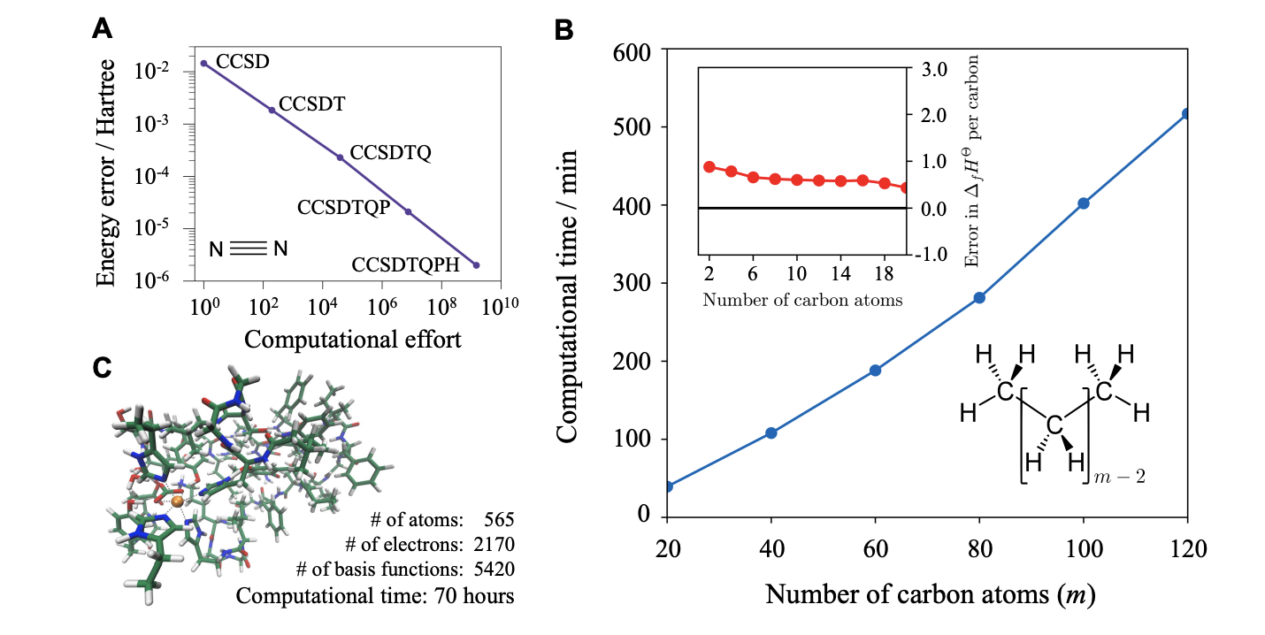
This might sound abstract, but the authors point out that coupled-cluster theory, which can (in principle) be extended to arbitrary levels of precision, can be made to take advantage of locality and scale linearly with increasing system size or increasing levels of accuracy. Although such algorithms aren’t known for strongly correlated systems, like metallic systems, Chan and co-workers argue based on analogy to strongly correlated model systems that analogous behavior can be expected.
Figure 3, showing linear scaling of coupled-cluster theory with respect to increasing accuracy (A) and increasing system size (B)
The above paper is making a very specific point—that exponential quantum advantage is unlikely—but doesn’t address whether weaker versions of quantum advantage are likely. Could it still be the case that quantum algorithms exhibit polynomial quantum advantage, e.g. scaling as O(N) while classical algorithms scale as O(N2)?
Another recent paper, from scientists at Google and QSimulate, addresses this question by looking at the electronic structure of various iron complexes derived from cytochrome P450. They find that there’s some evidence that quantum computers (using quantum phase estimation) will be able to outcompete the best classical methods today (CCSD(T) and DMRG), but it’ll take a really big quantum computer:
Most notably, under realistic hardware configurations we predict that the largest models of CYP can be simulated with under 100 h of quantum computer time using approximately 5 million qubits implementing 7.8 × 10⁹ Toffoli gates using four T factories. A direct runtime comparison of qubitized phase estimation shows a more favorable scaling than DMRG, in terms of bond dimension, and indicates future devices can potentially outperform classical machines when computing ground-state energies. Extrapolating the observed resource estimates to the full Cpd I system and compiling to the surface code indicate that a direct simulation of the entire system could require 1.5 trillion Toffoli gates—an unfeasible number of Toffoli gates to perform.
(A Toffoli gate is a three-qubit operator, described nicely here.)
A recent review agrees with this assessment: the authors write that “there is currently no evidence that heuristic NISQ approaches [like VQE] will be able to scale to large system sizes and provide advantage over classical methods,” and conclude with this paragraph:
Solving the electronic structure problem has repeatedly been identified as one of the most promising applications for quantum computers. Nevertheless, the discussion above highlights a number of challenges for current quantum approaches to become practical. Most notably, after accounting for the approximations typically made (i.e. incorporating the cost of initial state preparation, using nonminimal basis sets, including repetitions for correctness checking and sampling a range of parameters), a large number of logical qubits and total T/Toffoli gates are required. A major difficulty is that, unlike problems such as factoring, the end-to-end electronic structure problem typically requires solving a large number of closely related problem instances.
An important thing to note, which the above paragraph alludes to, is that the specific quantum algorithms discussed here don't actually make quantum chemistry faster than today’s methods—they typically rely on a Hartree–Fock ansatz, which is about the same amount of work as a DFT calculation. Since it's likely that proper treatment of electron correlation will require a sizable basis set, much like we see with coupled-cluster theory, we can presume that quantum methods would be slower than most DFT methods (even assuming that the actual quantum part of the calculation could be run instantly).
This ignores the fact that the quantum methods would of course give much better results—but an uncomfortable truth is that, unlike one might think from the exuberant press releases quoted above, classical algorithms generally do an exceptional job already. Most molecules are very simple from an electronic structure perspective: static electron correlation is pretty rare, and linear scaling CCSD(T) approaches are widely available and very effective (e.g.). There’s simply no need for FCI-quality results for most chemical problems, random exceptions notwithstanding.
(Aspuru-Guzik and co-workers agree; in a 2020 review, they state that they “do not expect [HF and DFT] calculations to be replaced by those on quantum computers, given the large system sizes that are simulated,” suggesting instead that quantum computers might find utility for statically correlated systems with 100+ spin orbitals)
A related point I made in a recent essay/white paper for Rowan is that quantum chemistry, at least as it’s applied to drug discovery, is limited not by accuracy but by speed. Existing quantum chemistry methods are already far more accurate than state-of-the-art drug discovery methods; replacing them with quantum computing-based approaches is like worrying about whether to bring a Lamborghini or a Formula 1 car to a go-kart race. It’s almost certain that there’s some way that “perfect” electronic structure calculations could be useful in drug design, but it’s hardly trivial to figure out how to turn a bunch of VQE calculations into a clinical candidate.
Other fields, like materials science, seem to be more limited by inaccuracies in theory—modeling metals and surfaces is really hard—but the Hartree–Fock ansatz is also hard here, and there are fewer commercial precedents for computational chemistry in general. To my knowledge, the Hartree–Fock starting point alone is a terrific challenge for a system like e.g. a cube of 10,000 metal atoms, which is why so many materials scientists avoid exact exchange and stick to local functionals. (I don't know much about computations on periodic systems, though, so correct me if this is wrong!) Using quantum computing to design superconducting materials probably won’t be as easy as it seems on Twitter/X.
So, while quantum computing is a terrifically exciting direction for computational chemistry in a scientific sense, I’m not sure it’s yet investable in a business sense. I don’t mean to belittle all the great scientific work being done in this field, in the papers I’ve referenced above and in many others. The point I’m trying to make here—that this field isn’t mature enough for actual commercial utility—could just as easily be made about ML in the 2000s, or any other number of promising but pre-commercial technologies.
I’ll close by noting that it seems like markets are coming around to this perspective, too. Zapata Computing, one of the original “quantum computing for chemistry” companies, recently pivoted to… generative AI, going public via a SPAC with Andretti (motorsport), and IonQ recently parted ways with its CSO, who is going back to his faculty job at Duke. We’ll see what happens, but progress in hardware has been slow, and it’s likely that it’ll be years yet until we can start to perform practical quantum chemical calculations on quantum computers.
In 2019, ChemistryWorld published a “wish list” of reactions for organic chemistry, describing five hypothetical reactions which were particularly desirable for medicinal chemistry. A few recent papers brought this back to my mind, so I revisited the list with the aim of seeing what progress had been made. (Note that I am judging these based solely by memory, and accordingly I will certainly omit work that I ought to know about—sorry!)
Fluorination
1. Fluorination – Exchanging a specific hydrogen for a fluorine atom in molecules with many functional groups. A reaction that installs a difluoromethyl group would be nice too.
This is still hard! To my knowledge, no progress has really been made towards this goal in a general sense (although plenty of isolated fluorination reactions are still reported, many of which are useful).
C–H fluorination is particularly challenging because separating C–H and C–F compounds can be quite difficult. (Fluorine is often considered a hydrogen bioisostere, which is nice from a design perspective but annoying from a chromatography perspective.) For this reason, I’m more optimistic about methods that go through separable intermediates than the article’s author: “installing another reactive group… and exchanging it for fluorine” may not be particularly ideal in the Baran sense, but my guess is that this strategy will be more fruitful than direct C–H fluorination for a long while yet.
Heteroatom Alkylation
2. Heteroatom alkylation – A reaction that – selectively – attaches an alkyl group onto one heteroatom in rings that have several, such as pyrazoles, triazoles and pyridones.
This problem is still unsolved. Lloyd-Jones published some nice work on triazole alkylation a few weeks after the ChemistryWorld article came out, but otherwise it doesn’t seem like this is a problem that people in academia are thinking much about.
Unlike some of the others, this challenge seems ideally suited to organocatalysis, so maybe someone else in that subfield will start working on it. (Our work on site-selective glycosylation might be relevant?)
EDIT: I missed extremely relevant work from Stephan Hammer, which uses engineered enzymes to alkylate pyrazoles with haloalkanes (and cites the ChemistryWorld article directly). Sorry!
Csp3 Coupling
3. Carbon coupling – A reaction as robust and versatile as traditional cross coupling for stitching together aliphatic carbon atoms – ideally with control of chirality, too. Chemists also want more options for the kinds of molecules they can use as coupling precursors.
There’s been a ton of work on Csp3 cross coupling since this article came out: MacMillan (1, 2, 3, 4, 5, 6) and Baran (1, 2, 3) have published a lot of papers, and plenty of other labs are also working here (I can’t list everyone, but I’ll highlight this work from Sevov). I doubt this can be considered “solved” yet, but certainly things are much closer than they were in 2019.
(I haven’t seen much work on enantioselective variants, though: this 2016 paper and paper #2 from Baran above are the only ones that comes to mind, although I’m sure I’m missing something. Still—an opportunity!)
Reactions of Heterocycles
4. Making and modifying heterocycles – A reaction to install functional groups – from alkyl to halogen – anywhere on aromatic and aliphatic heterocycles, such as pyridine, piperidine or isoxazole. Reactions that can make completely new heterocycles from scratch would be a bonus.
I’m not a big fan of the way this goal is written—virtually every structure in medicinal chemistry has a heterocycle, so “making and modifying heterocycles” is just too vague. What would a general solution even look like?
Nevertheless, there are plenty of recent papers which address this sort of problem. Some of my favorites are:
Aaron Sather’s work making N-aryl piperidines (1, 2)
Some nice reagent design from Patrick Fier, which basically improves on the Chichibabin reaction
(One of my friends in academia told me that they really disliked the Sather work because it was just classic reactivity used in a straightforward way, i.e. not daring enough. What a clear illustration of misaligned incentives!)
Atom Swapping/Skeletal Editing
5. Atom swapping – A reaction that can exchange individual atoms selectively, like swapping a carbon for a nitrogen atom in a ring. This chemical version of gene editing could revolutionise drug discovery, but is probably furthest from realisation.
Ironically, this goal is probably the one that’s closest to realization today (or perhaps #3): Noah Burns and Mark Levin have both published papers converting benzene rings directly to pyridines recently. More broadly, lots of organic chemists are getting interested in “skeletal editing” (i.e. modifying the skeleton of a molecule, not the periphery), which seems like exactly what this goal is describing. To my knowledge, a comprehensive review has not yet been published, but this article gives a pretty good overview of the area.
Overall, it’s impressive how much progress has been made towards the goals enumerated in the original article, given that it’s only been four years (less than the average length of a PhD!). Organic methodology is a very exciting field right now: data is easy to acquire, there are lots of problems to work on, and there seems to be genuine interest from adjacent fields about the technologies being developed. Still, if the toughest challenges in the field’s imagination can be solved in under a decade, it makes you wonder what organic methodology will look like in 20–30 years.
As methods get faster to develop and more and more methods are published, what will happen? Will chemists employ an exponentially growing arsenal of transformations in their syntheses, or will the same methods continually be forgotten and rediscovered every few decades? Will computers be able to sift through centuries of literature and build the perfect synthesis—or will the rise of automation mean that we have to redesign every reaction to be “dump and stir”? Or will biocatalysis just render this entire field obsolete? The exact nature of synthesis’s eschatology remains to be determined.
Scientists, engineers, and other technical people often make fun of networking. Until a few years ago, I did this too: I thought networking was some dumb activity done by business students who didn’t have actual work to do, or something exploitative focused on pure self-advancement. But over the past year or so, I’ve learned why networking is important, and have found a way to network that doesn’t make me feel uncomfortable or selfish. I want to share my current thoughts here, in case they help anyone else.
The first thing to recognize is that networking matters because we live in a world of relationships. Technical people often struggle with this point: to some, relying on relationships feels imprecise or even nepotistic. But we’re human beings, not stateless automata communicating via some protocol, and it’s inevitable (and appropriate) for us to form relationships and care about them.
Having the right relationships can make a big difference. We trust people we know much more than we trust strangers. It’s weird for someone whom you’ve never met to email you asking for a favor, but very normal for a friend or acquaintance to reach out and ask for something. And most ambitious projects (academia, startups, etc) are limited not by money but by human capital: there are only so many talented people out there, and if you can’t get access to them, what you’re doing will suffer. (On a macro level, this explains why management consulting has become so important.)
So it’s worth intentionally building relationships before you have an immediate need. There are a lot of people,[citation needed] so how might one go about this? One obvious strategy might be to build relationships with people you think could be useful to you. But this doesn’t work very well. It’s not always obvious what will or won’t be useful in the future, and far too easy to let status quo bias reign supreme. (Most graduate students struggle to imagine how knowing someone from another subfield could ever be useful, let alone someone who isn’t a scientist, which makes it tough when they want to do something outside academia.)
Another downside to this strategy is that you have to partition people into “useful” or “not useful” upon meeting them. This is self-defeating: most people can figure out when you’re treating them only as a means to an end, so walking around evaluating everyone’s utility tends to poison your interactions. Plus, it’s a very Machiavellian way to view the world, and ought to make you feel a little gross.
Instead, a better strategy is to accept that you won’t be able to predict a priori who will be useful and instead just try and meet people. If the end goal of networking is to find people you’ll be able to collaborate with in the future, in one capacity or another, then it’s important to find people who share your values and who you get along with: in other words, friends. So, rather than worrying about if it’ll be better to know a renewable energy consultant or a paralegal for a medical device company, you can just see who you like spending time with and go from there.
If we think of networking as synonymous to making friends, then it also becomes more obvious when and how one should network. Anything explicitly framed as an opportunity for networking is a bad choice: these events tend to attract people who are self-centered, and mostly end up revolving around LinkedIn (the Tinder of networking?). Instead, look for places where you’ll find people you could be friends with. For me, this ends up mostly being church and church-adjacent spaces like Bible studies; I’m not sure what the analogous space for non-religious people is.
The strategies I’ve discussed above are framed in terms of “demand-side networking,” or how you can find ways to acquire human capital when you have a demand for it. But the same considerations apply to “supply-side networking,” or marketing oneself to potential people. The beauty of treating networking simply as making friends is that you’re not committing to any particular outcome: maybe you’ll benefit from it, maybe the other person will benefit from it, or maybe both of you will (or neither). The expected value of building new relationships should always be positive, which means that networking isn’t a zero-sum game: it’s good for all involved.
The conclusion I want to leave you with is this: networking, rightly understood, just means living in a way that recognizes our dependence on other people. To live life as a “networker” means putting yourself in places where you might make new friends, looking for common ground in all your interactions, and trying to recognize others’ talents and abilities. Networking isn’t some Randian pursuit focused on extracting value from those around us. It should be done with humility, accepting that we need other people to thrive and being open to whatever relationships come our way.
Thanks to Ari Wagen for editing drafts of this post.