Apologies for the long hiatus: we've had some health issues in the family, and startup life has been particularly overwhelming. With any luck, I'll be able to return to a more regular posting frequency soon.
What’s the right relationship between theory, computation, and experiment? Much has been written on this. In this piece, I want to put forward an answer that I think is underrated in the life sciences—what I call the “SolidWorks model” of simulation.
For the unfamiliar, SolidWorks is a program which allows engineers to design objects in the computer: the user can create a 3D model of their device, figure out the measurements that allow the parts to fit together in the desired way, and then go into the lab and actually build everything. (I’m not a SolidWorks power user, but I spent a semester messing around with it in high school and I’ve been thinking back on this recently.)
A screenshot of SolidWorks.
What are the distinctive features of SolidWorks?
SolidWorks doesn’t predict overall success. If you’re designing a new gearbox in SolidWorks, you can check that the parts will fit together, but you don’t know if it will run efficiently or not. Modeling is not supposed to replace actually building and testing the part.
SolidWorks can be used by normal engineers, not dedicated computer experts. It’s quick and easy to model things, so modeling becomes a part of the regular engineering/design workflow. You can model a part, make it, adjust the model, make it again, and so on and so forth.
SolidWorks assists human intuition instead of trying to replace it. SolidWorks only draws what you tell it to, which means all the ideas still come from humans—to the extent that SolidWorks increases productivity, it does so by helping people understand what they’re working on more clearly. This comports with Richard Hamming’s idea that “the purpose of computing is insight, not numbers.”
Astute readers will notice differences from how simulations in the life sciences are typically conducted. It’s rare in chemistry or biology to have computations and experiments performed in the same research group, let alone by the same person—but this is crucial to SolidWorks-style simulation, where experimental scientists must quickly gain insight from their computations. If someone from a different team has to get around to answering their request or a job takes overnight to run, the experimental scientist will move on and modeling will be excluded from the design/build/test cycle.
SolidWorks-style computation is also prospective, not retrospective. In other words, the goal of the simulation is to generate subsequent experimental hits, not figures for publication, meaning that successful computational studies might never even be reported. This is different from the DFT section of the average organic chemistry paper, which is typically performed by a different team after all experimental results are complete. This isn’t bad, but ex post studies are different from actually using computations ex ante to design molecules.
I don’t mean to suggest that the SolidWorks paradigm is objectively correct: there are many ways in which theory, computation, and experiment can usefully interact, and I think it’s great that there are scientists using careful ex post computations to interpret perplexing experimental results or running massive virtual screens to design new molecules entirely in silico. I myself have worked on plenty of projects like this and hope to conduct more in the future.
But I do think that SolidWorks-style computation is pretty underrated today. There are few computational tools that non-experts can really use, and the average experimental scientists might not interact with computation even once in an average week (except perhaps when meeting with someone from a different lab or team). Even when experimentalists have the technical skills to run calculations, the friction involved in connecting to a computing cluster, generating input files, monitoring jobs, etc often makes it impractical to really run calculations and experiments in tandem.
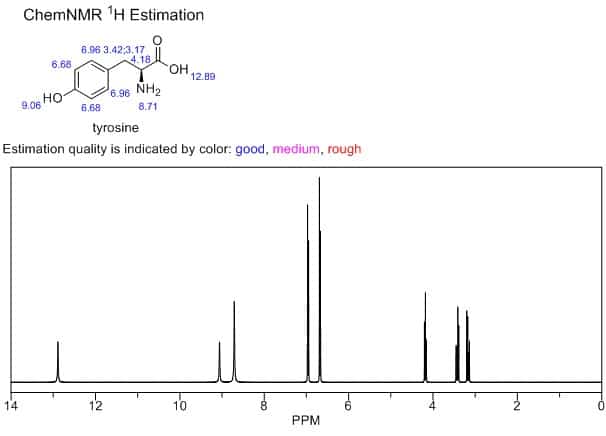
In fact, I’d argue that the most useful predictive computational tool for organic chemists has probably been the ChemDraw “Predict NMR” button. The predictions are laughably crude by today’s standards, but ChemDraw NMR has a few key advantages: (1) you don’t have to program anything or look at a terminal window to use it, (2) there aren’t any options for end users to mess around with, so you can’t do anything wrong, and (3) it runs instantly from a software package everyone already has, so it fits right into your workflow. These factors are collectively more important than accuracy—ChemDraw NMR is accurate enough to be useful, and far more convenient than fancier approaches.
A screenshot of ChemDraw's NMR prediction widget.
This seems like a scenario where publication pressure leads to misaligned incentives. Scientific publications emphasize novelty, accuracy, and performance, not pragmatic considerations like “how easy is it to run this software in the middle of the workday” or “how confusing are the parameters to understand.” And for pioneering computational workflows that ought not to be run without a deep understanding of the science, that’s probably appropriate. But pragmatic considerations matter for casual users.
If it’s not obvious by now, one of our big visions for Rowan is “SolidWorks for organic chemistry”—to the extent that there are people who are designing and creating new molecules, we think that it’s important that they are able to think intelligently about the molecules that they’re designing. This means making software that can deliver actionable insights while being fast and simple enough for experimentalists to use. While this is a massive project, it’s not impossibly large, and we’re optimistic that Rowan can quickly become helpful to experimental chemists. If you think this vision is exciting and have ideas for how we can bring it to life, let us know!
“POC has evolved in many directions and its concepts are widely used, e.g., in host-guest chem, org syn, materials sci, drug discovery.” - Bill Jorgensen
“There is still a lot of absolutely gorgeous classical phys org done with organometallic and enzymatic reactions. The molecules have changed, the ideas are the same.” - Dan Singleton
“It makes no sense. Looking at orbitals, measuring KIE, studying mechanisms, all traditional PhysOrgChem. And ML in OrgChem is nothing more than Curtin-Hammett on steroids.” - Sebastian Kozuch
“Hard core classical phys-org maybe, but structure-activity relationships are alive and well across all chemistry disciplines. These have their origin in phys-org and use so many fundamental principles I learned as a PhD student studying carbocation and free radical reactions.” - @RacerPolyLab
“I've attend 10 Phys Org GRC meetings since 1999 & chaired 2015. I'm OK with ‘traditional phys. org. chemistry’ being barely practiced. It was dying–2001 saw 79 attendees, then the area morphed into phys. org. of organometallics, supramolecular, biomolecules. Fields evolve or die.” - Michael Haley
(There are plenty more responses; if I didn’t list yours, sorry!)
For the most part, I agree with these responses. Physical organic thinking has permeated organic chemistry and adjacent fields: George Whitesides has probably the best piece on this topic, in which he argues that the essence of physical organic chemistry is “a general, and remarkably versatile, method for tackling complex problems,” not anything about chemistry per se, and consequently that the physical organic mindset can be applied to problems in all manner of fields. Viewed from this angle, we might say that physical organic chemistry hasn’t disappeared at all—instead, it’s become so commonplace that we forget to acknowledge it as distinctive at all.
Looking through the organic chemistry curriculum, too, suggests that physical organic chemistry is here to stay. Lots of the ideas that we teach to undergraduates, like molecular orbital theory and structure–activity relationships, were once distinctively the domain of physical organic chemists. Textbooks from before the apotheosis of physical organic chemistry (I have an old copy of Fieser & Fieser, for instance) are structured in a completely different way, not by mechanism but by functional group, while today many undergraduate organic classes discuss SN1/SN2 mechanisms in their first semester.
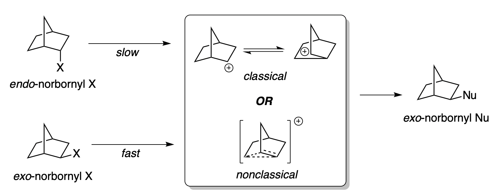
So, was I entirely wrong to claim that traditional physical organic chemistry is a dying art? I don’t think so. Despite all the successes of physical organic chemistry, it seems to me that something has been lost between the time of the norbornyl cation controversy and today. The sorts of elegant kinetic experimentation and argumentation that Winstein and others employed in their papers are now rare: take, for instance, this famous paper distinguishing between contact ion pairs and solvent-separated ion pairs. How many scientists today still do experiments like this? There are certainly names that come to mind, but from where I sit it seems to be an increasingly niche skillset.
I don’t want to fall into the trap of idolizing the past for no reason; there are plenty of techniques which have been forgotten by chemistry because there are better ways of doing the same thing today. Chemists used to estimate molecular weight by dissolving a known mass of sample and measuring the boiling point elevation induced. Now we have mass spectrometry, so nobody uses the boiling point method any more, and I don’t see this as a great tragedy.
But kinetics, and more generally the sort of careful physical organic chemistry practiced by participants in the norbornyl cation debate, doesn’t seem to have such a simple replacement. Computation is the most obvious candidate, but we’re still a long way away from being able to predict mechanisms accurately in silico; in mechanistic chemistry, experiments still reign supreme. Kinetic isotope effects are much easier to measure than they were back in Winstein’s day, but they’re hardly routine experiments (and easy to get wrong). The rigor and precision with which old-school physical organic chemistry approached mechanistic problems can still be found today, but it seems harder and harder to find.
It might have been inevitable that physical organic chemistry was always going to evolve away from incredibly detailed studies of simple reactions on simple molecules—just as biology has largely shifted from ecology and taxonomy to cell biology and biochemistry, organic chemistry too must change in order to keep working on the most interesting problems. And perhaps there's some truth to the argument that the old-school style of painstaking mechanistic study just isn't worth the effort and deserves to be de-emphasized. But it does seem to me that parts of the tradition of physical organic knowledge (to borrow Samo Burja’s phrasing) is being slowly lost to time, despite the fact that lots of really good physical organic chemistry is still being done today on all sorts of problems (enzymatic chemistry, organometallic chemistry, catalysis, heterogenous catalysis, chemical biology, &c), and that makes me sad.
In this post, I’m trying something new and embedding calculations on Rowan alongside the text. You can view the structures and energies right in the page, or you can follow a link and view the full data in a new tab. While PDFs and printed journals are limited to displaying 2D renditions of 3D structures, there’s no reason why websites should follow suit—and now that all my calculations are already on the web, it’s simple to share the primary data.
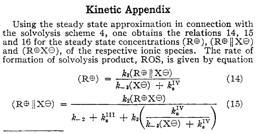
The 2-norbornyl cation has a special place in the history of physical organic chemistry. In 1949, following up on previous work by Christopher Wilson, the great physical organic chemist Saul Winstein observed that acetolysis of exo-norbornyl sulfonates occurred about 350 times faster than solvolysis of the corresponding endo compounds.
“X” represents a leaving group and “Nu” a nucleophile.
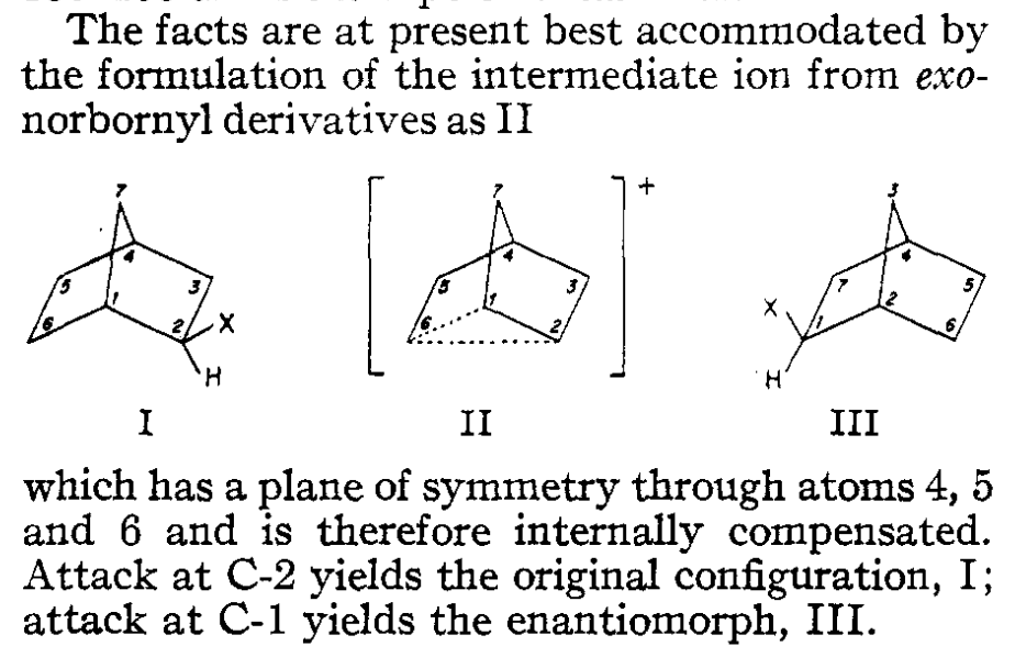
Several stereochemical observations indicated that something puzzling was going on: both the exo and endo sulfonates gave exo acetate product, but enantioenriched exo-norbornyl sulfonate formed racemic exo-norbornyl acetate. Winstein argued that this data was best explained through the participation of an achiral nonclassical carbocation (“II”) featuring σ-delocalization and a three-center two-electron bond, as shown in the conclusion of the 1949 paper:
The nonclassical structure, “II” above, is a little tough to visualize as drawn. Here’s the computed structure at the B3LYP-D3BJ/6-31G(d) level of theory, which should be a bit clearer. You can click on atoms to see bond distances, angles, and dihedrals; notice that the C1–C2 bond above (C14–C18 in Rowan) is markedly shorter than a normal C–C bond, whereas the C1–C6 and C2–C6 bonds (C13–C14 and C14–C18 in Rowan) are quite long.
In the 1960s Winstein’s interpretation was challenged by another preeminent chemist, H.C. Brown, who argued that the data could adequately be explained by rapidly equilibrating classical carbocations. Brown suggested that most of the observations made by Winstein could be explained simply by the differing steric profiles of the exo and endo faces of the norbornyl cation: the endo face is more shielded, and so ionization is slowed (explaining the 350:1 exo/endo rates) and attack is disfavored (explaining why both isomers of sulfonate give exo product).
This began an incredibly contentious series of debates which dragged on for decades. Rather than attempt to wade through the resulting sea of publications, I’ll quote from an excellent 1983 review by Cheves Walling to give a sense for the magnitude of the controversy:
The debate [over the structure of the norbornyl cation] was vigorously pursued verbally in lectures, meetings, and seminars all over the U.S. and even abroad…. No one has ever counted the number of publications touching on the 2-norbornyl cation problem, but they include a number of reviews, chapters, and books, and a typcial [sic] research paper may well include references to over 100 others.
Walling’s review goes on to give an excellent overview of the various pieces of evidence employed by both sides of the debate, which I won’t summarize in full here.
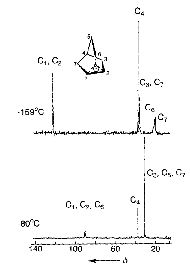
The most important data was obtained by George Olah and co-workers, who pioneered the use of superacidic media to generate stable solutions of carbocations which could be characterized spectroscopically. With Martin Saunders and others, Olah employed 1H and 13C NMR spectroscopy, IR spectroscopy, Raman spectroscopy, and core electron spectroscopy to study low-temperature solutions of norbornyl cations: in all cases, the data supported Winstein’s proposed symmetric structure. (While equilibration occurring faster than the spectroscopic timescale could not be ruled out by Olah’s work, spectroscopic measurements all the way down to 5 K showed no detectable classical structures, indicating that any barrier to interconversion must be <0.2 kcal/mol.)
13C NMR spectra at –159 ºC, showing the equivalence of C1 and C2. At –80 ºC, rapid Wagner–Meerwein rearrangements render C1, C2, and C6 equivalent.
Data taken from Olah's Nobel lecture.
(This is a good use case for carbon NMR!)
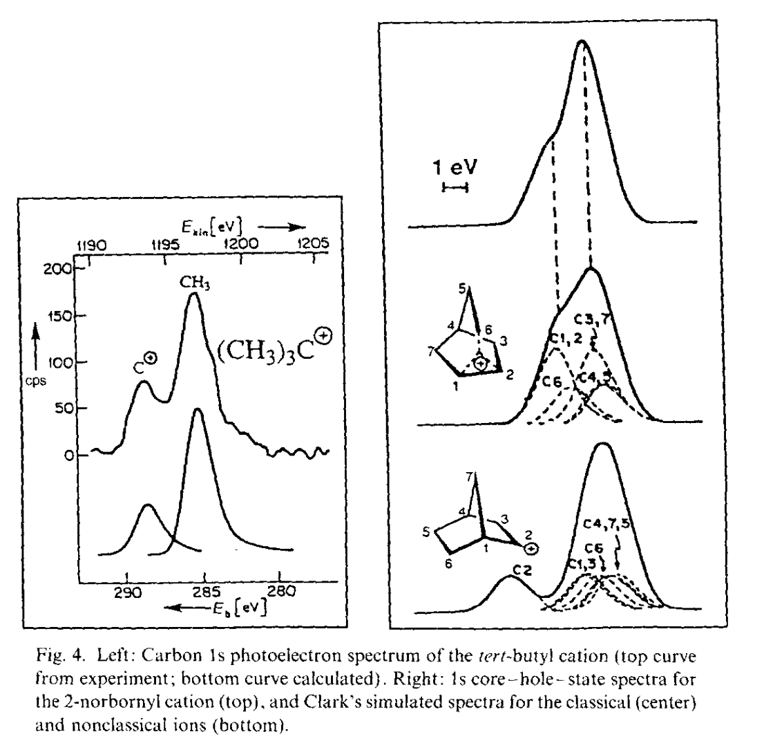
Carbon 1s photoelectron spectrum of tert-butyl carbocation (left), showing a characteristic carbenium peak on the left, and the analogous spectrum for the norbornyl cation showing the absence of the carbenium peak. Data taken from Olah's Nobel lecture.
Computational chemistry, which became able to tackle problems like this in the late 1980s and early 1990s, also supported the nonclassical structure of the norbornyl cation. A 1990 paper used HF/6-31G(d) calculations in Gaussian 86 to show that the symmetric structure was a minimum on the potential energy surface. Here’s a scan I ran at the B3LYP-D3BJ/6-31G(d) level of theory, showing that the energy increases as the “classical” C–C bond forms:
(This iframe doesn't work well on the phone - still a work in progress, sorry.)
Subsequent work has confirmed that Winstein was almost completely correct about the key issues. Most notably, a 2013 crystal structure from Karsten Meyer demonstrates that the norbornyl cation is indeed nonclassical in the ground state, leading Chemistry World to declare the mystery solved. Nevertheless, there’s still a little room for a classical cation supporter to doubt this result: crystal structures are snapshots of solid-state atomic configurations, while reactions occur in solution, where molecules are free to move around more. (In the Chemistry World article, Paul Schleyer predicts that Brown himself would have raised this objection.)
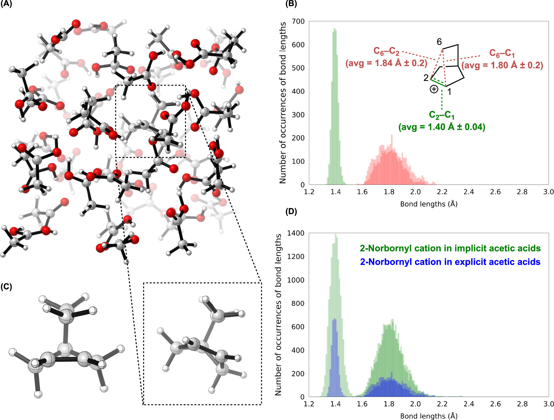
A paper from Ken Houk and co-workers, published a few days ago in JOC, addresses this issue by directly modeling the solvolysis process through ab initio molecular dynamics with explicit acetic acid solvent. In the solvolysis of the exo sulfonate, the authors find the nonclassical cation is formed on average within 9 femtoseconds of C–O bond cleavage, which is about as quickly as is physically possible. Once formed, the cation is entirely nonclassical: “classical 2-norbornyl cations are a negligible component of norbornyl cations in solution," thus addressing the last objection of classical cation partisans.
Simulations of the norbornyl cation in explicit acetic acid show complete nonclassical behavior (Figure 6 from Houk’s paper).
In contrast, Houk et al find that the endo sulfonate doesn’t form the nonclassical cation until about 81 fs after the C–O bond breaks, explaining the slower reaction rate: the transition state isn’t stabilized by σ-dissociation, and so is higher in energy. This is a nice example of the principle of nonperfect synchronization, which is explained concisely in this presentation.
What can modern scientists learn from the norbornyl cation controversy, besides the object-level fact that carbocations can exhibit nonclassical σ-delocalization?
1. Reality is confusing, and convincing arguments are often wrong.
It’s a good exercise to go back and read the early H.C. Brown papers in this area, like this account. Brown was an incredible scientist (the 1979 Nobel laureate in chemistry), and his data and reasoning are quite good; I find myself sympathizing with his viewpoint while reading his papers. Nevertheless, with the benefit of hindsight we know that he was wrong and Winstein was right. “Humility comes before honor.”
2. Tools drive scientific progress.
The argument over the norbornyl cation was ultimately settled only by the development of new techniques, like superacid chemistry, core electron spectroscopy, and high-level calculations. Now that we have these methods, it’s much easier to solve similar problems: if Winstein’s paper came out today, I doubt it would take more than a year or two to figure everything out.
This aligns nicely with what Freeman Dyson calls a “Galisonian” view of scientific progress, where scientific progress is driven not by ideas (the “Kuhnian” view) but by new tools and new data. In chemistry, at least, the tools-first view seems true to me—since 1950, it’s difficult to think of a development more important to organic chemistry than NMR spectroscopy, with flash column chromatography probably taking second place.
3. It’s easy for fields to get distracted by controversy and lose relevance.
Here’s Walling again:
Since a significant fraction of the efforts of physical organic chemists was drawn into the problem [of the norbornyl cation], an unhappy consequence was a feeling on the part of many (including some of those concerned with the distribution of research funds) that physical organic chemistry was in danger of withdrawing into a world of its own.
As older scientists have explained to me, the norbornyl cation debacle scared a generation of chemists away from physical organic chemistry. The entire subfield became obsessed with a niche and somewhat irrelevant issue, while scientists in adjacent subfields looked on with bemusement and frustration. As a consequence, traditional physical organic chemistry is barely practiced today: few scientists have the skill or knowledge to conduct kinetic studies like those performed by Winstein, Brown, and others, and those still working in the area struggle to get funding or recognition (in the words of Dan Singleton, “sucks when you have to peddle your papers in cemeteries”).
(In a nice historical perspective, Stephen Weininger argues the norbornyl cation debate was “a hook on which to hang a much larger agenda,” fueled both by a UK/US divide and a deeper dispute about whether valence bond representations or molecular orbital representations of chemical structures were superior. If this is true, it was a self-defeating exercise by all involved.)
Scientists should be motivated by a search for truth, but also by the desire to improve the world. Usually these two aims go together: basic research without obvious societal implications often leads to unexpected and important findings, which is why the government supports science in the first place. But it’s possible to become so myopically focused on a single issue in the name of truth that one forgets about other goals, as arguably happened in the norbornyl cation imbroglio.
Controversy attracts attention: we’re drawn to it, against our better judgment, like moths to a flame. We have to be careful not to get captured by disputes that are, in the long run, not worth the effort.
Thanks to Eric Jacobsen for many conversations about the history of physical organic chemistry, Eugene Kwan for conversations about the principle of nonperfect synchronization, and to Ari Wagen for feedback on this post and six months of excellent front-end development for Rowan. Any errors are mine alone.
#1. Tony Fadell, Build #2. Giff Constable, Talking To Humans #3. Ben Horowitz, The Hard Thing About Doing Hard Things #4. Dale Carnegie, How To Win Friends And Influence People
Sounds Machiavellian, but actually quite wholesome: a “dad book,” as my friend called it.
#5. Ben Patrick, Knee Ability Zero.
#6. Neal Stephenson, The Diamond Age
Snow Crash was much worse upon rereading as an adult, but The Diamond Age was a bit better: in particular, I didn’t really appreciate the “speculative governance futurism”/”comparative cultural criticism” facets of the novel when I read this in high school.
#7. Richard Hamming, The Art of Doing Science and Engineering
Many great works of literature are notable for their brevity: when you read Hemingway, or Dubliners, or Flannery O’Connor, you know that every sentence has been crafted with care. Giant fantasy novels like Wheel of Time (which I read last year) or The Stormlight Archives work differently. There are entire chapters which are probably extraneous, whole characters and plot arcs which exist merely to bring out certain traits or pieces of information.
But there are unique joys to megafiction: sitting down and reading hundreds of pages of a good story is relaxing in a way that other books simply aren’t. In my own life, I’ve found that I’m much better about making time to read when I’m in the middle of an engaging novel than when I’m reading theology or histories of feudalism. Narrative-driven “easy reading” has a bad reputation amongst the literati; in a world where all fiction is competing against screens for engagement, it shouldn’t.
#13. Tom Holland, Rubicon #14. Tom Holland, Dynasty #15. Czeslaw Milocz, The Captive Mind
Fantastic; I probably would have liked this even more if I were still in school.
#16. C.S. Lewis, That Hideous Strength
I didn’t like this when I was a kid, but I like it now: in many respects THS can be viewed as a book-length exploration of the ideas in “The Inner Circle,” with a garnish of medieval cosmology here and there (see also).
#17. Kazuo Ishiguro, Klara and the Sun #18. Mike Cosper, Recapturing the Wonder #19. Mairtin O Caidhan, Graveyard Clay
Tyler Cowen recommended this book, but I didn’t love it.
#20. Ursula K. LeGuin, The Dispossessed #21. Marty Cagan, Inspired #22. Ernst Junger, On the Marble Cliffs
The best book I read this year by a mile; far better than I remembered. While many of The Canterbury Tales work pretty well as literature, they’re even better when viewed also as history. It’s rare to be able to read something from 800 years ago that’s legitimately funny and interesting.
Reading Chaucer fills me with questions about the medieval mind. The stories are steeped in Christianity, as one might expect. Any argument goes back to the Bible, even those among animals, and Chaucer assumes a level of familiarity with e.g. the Psalms far exceeding that of most modern Christians. Yet at the same time the Greco-Roman world looms large: Roman gods appear as plot characters in three tales (the Knight’s Tale, the Merchant’s Tale, and the Manciple’s Tale), and Seneca is viewed as a moral authority on par with Scripture. I’m curious how all these beliefs and ideas fit together and welcome any recommendations on this subject. (The Discarded Image is already on my list.)
#27. Gabrielle Zevin, Tomorrow and Tomorrow and Tomorrow
My wife recommended this book to me. I thought this would be a relaxing break from the November startup grind, but in fact it features a bunch of obsessed programmers working around the clock for months—a poor choice but a good novel.
#28. Jessica Livingston, Founders at Work #29. Neal Stephenson, Seveneves
Overall, about a third of the books I read were startup-related: most of them were pretty bad, but even bad business/startup books are probably useful from the viewpoint of cultural immersion. Academic science is quite different from the startup ecosystem, and to the extent that cultural arbitrage is possible (in either direction), I need to become proficient in startup culture.
I’m not sure why the median business book is so bad—perhaps business people are too willing to spend money on books and not picky enough, or perhaps MBA types generally lack knowledge about the humanities, which makes both supply and demand worse.
(The median Christian book is also pretty bad. One unifying hypothesis: both pastors and businesspeople often have wise insights into specific situations, personal or business, but these insights aren’t readily generalizable into book form. Being able to give good advice doesn’t mean you should write an “advice book.”)
As always, book recommendations are welcome, particularly on the topics of medieval history/culture, software engineering, or startups. Apologies for the infrequent posting as of late, and happy new year!
“And I took the little scroll from the hand of the angel and ate it. It was sweet as honey in my mouth, but when I had eaten it my stomach was made bitter.”
–Revelation 10:10
As machine learning becomes more and more important to chemistry, it’s worth reflecting on Richard Sutton’s 2019 blog post about the “bitter lesson.” In this now-famous post, Sutton argues that “the biggest lesson that can be read from 70 years of AI research is that general methods that leverage computation are ultimately the most effective, and by a large margin.” This might sound obvious, but it’s not:
[The bitter lesson] is a big lesson. As a field, we still have not thoroughly learned it, as we are continuing to make the same kind of mistakes. To see this, and to effectively resist it, we have to understand the appeal of these mistakes. We have to learn the bitter lesson that building in how we think we think does not work in the long run. The bitter lesson is based on the historical observations that 1) AI researchers have often tried to build knowledge into their agents, 2) this always helps in the short term, and is personally satisfying to the researcher, but 3) in the long run it plateaus and even inhibits further progress, and 4) breakthrough progress eventually arrives by an opposing approach based on scaling computation by search and learning. The eventual success is tinged with bitterness, and often incompletely digested, because it is success over a favored, human-centric approach.(emphasis added)
How might the bitter lesson be relevant in chemistry? One example is computer-assisted retrosynthesis in organic synthesis, i.e. figuring out how to make a given target from commercial starting materials. This task was first attempted by Corey’s LHASA program (1, 2), and more recently has been addressed by Bartosz Gryzbowski’s Synthia. Despite considerable successes, both efforts have operated through manual encoding of human chemical intuition. If Sutton is to be believed, we should be pessimistic about the scalability and viability of such approaches relative to pure search-based alternatives in the coming years.
Another example is machine-learned force fields (like ANI or NequIP). While one could argue that equivariant neural networks like e3nn aren’t so much incorporating domain-specific knowledge as exploiting relevant symmetries (much like convolutional neural networks exploit translational symmetry in images), there’s been a movement in recent years to combine chemistry-specific forces (e.g. long-range Coulombic forces) with neural networks: Parkhill’s TensorMol did this back in 2018, and more recently Dral, Piquemal, and Levitt & Fain (among others) have published on this as well. While I’m no expert in this area, the bitter lesson suggests that we should be skeptical about the long-term viability of efforts, and instead just throw more data at chemistry-agnostic models.
A key assumption of the bitter lesson is that “over a slightly longer time than a typical research project, massively more computation inevitably becomes available.” This idea has also been discussed by Andrej Karpathy, who reproduced Yann LeCun’s landmark 1989 backpropagation paper last year using state-of-the-art techniques and reflected on how the field has progressed since then. In particular, Karpathy discussed how the last three decades of progress in ML can help us envision what the next three decades might look like:
Suppose that the lessons of this exercise remain invariant in time. What does that imply about deep learning of 2022? What would a time traveler from 2055 think about the performance of current networks?
2055 neural nets are basically the same as 2022 neural nets on the macro level, except bigger.
Our datasets and models today look like a joke. Both are somewhere around 10,000,000X larger.
One can train 2022 state of the art models in ~1 minute by training naively on their personal computing device as a weekend fun project.
Today’s models are not optimally formulated, and just changing some of the details of the model, loss function, augmentation or the optimizer we can about halve the error.
Our datasets are too small, and modest gains would come from scaling up the dataset alone.
Further gains are actually not possible without expanding the computing infrastructure and investing into some R&D on effectively training models on that scale.
If we take this seriously, we might expect that chemical ML will not be able to advance much farther without bigger datasets and bigger models. Today, experimental datasets rarely exceed 104–105 data points, and even computational datasets typically comprise 107 data points or fewer—compare this to the ~1013 tokens reportedly used to train GPT-4! It’s not obvious how to get experimental datasets that are this large. HTE and robotics will help, but five orders of magnitude is a big ask. Even all of Reaxys doesn’t get you to 108, poor data quality notwithstanding. (It’s probably not a coincidence that DNA-encoded libraries, which can actually have hundreds of millions of data points, also pair nicely with ML: I’ve written about this before.)
In contrast, computation permits the predictable generation of high-quality datasets. If Sutton is right about the inevitable availability of “massively more computation,” then we can expect it to become easier and easier to run hitherto expensive calculations like DFT in parallel to generate huge datasets, and to enable more and more downstream applications like chemical machine learning. With the right infrastructure (like Rowan, hopefully), it should be possible to turn computer time into high-quality chemical data with almost no non-financial scaling limit: we’re certainly not going to run out of molecules.
The advent of big data, though, heralds the decline of academic relevance. Julian Togelius and Georgios Yannakakis wrote about this earlier this year in a piece on “survival strategies for depressed AI academics,” which discusses the fact that “the gap between the amount of compute available to ordinary researchers and the amount available to stay competitive is growing every year.” For instance, GPT-4 reportedly cost c. $60 million to train, far surpassing any academic group’s budget. Togelius and Yannakakis provide a lot of potential solutions, some sarcastic (“give up”) and others quite constructive—for instance, lots of interpretability work (like this) is done on toy models that don’t require GPT-4 levels of training. Even the most hopeful scenarios they present, however, still leave academics with a rather circumscribed role in the ML ecosystem.
The present academic era of chemical machine learning can thus be taken as a sign of the field’s immaturity. When will chemical ML reach a Suttonian era where scaling is paramount and smaller efforts become increasingly futile? I’m not sure, but my guess is that it will happen when (and only when) there are clear commercial incentives for developing sophisticated models, enabling companies to sink massive amounts of capital into training and development. This clearly hasn’t happened yet, but it also might not be as far away as it seems (cf.). It’s an interesting time to be a computational chemist…