
“A cord of three strands is not easily broken.”
Computational chemistry, like all attempts to simulate reality, is defined by tradeoffs. Reality is far too complex to simulate perfectly, and so scientists have developed a plethora of approximations, each of which reduces both the cost (i.e. time) and the accuracy of the simulation. The responsibility of the practitioner is to choose an appropriate method for the task at hand, one which best balances speed and accuracy (or to admit that no suitable combination exists).
This situation can naturally be framed in terms of Pareto optimality: there’s some “frontier” of speed/accuracy combinations which are at the limit of what’s possible, and then there are suboptimal combinations which are inefficient. Here’s a nice plot illustrating exactly that, from Dakota Folmsbee and Geoff Hutchinson (ref):
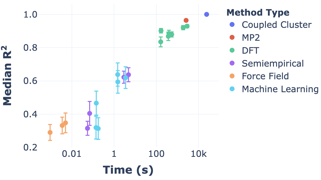
In this figure, the top left corner is the goal—perfect accuracy in no time at all—and the bottom right corner is the opposite. The diagonal line represents the Pareto frontier, and we can see that different levels of theory put you at different places along the frontier. Ab initio methods (DFT, MP2, coupled cluster) are slow but accurate, while force fields are fast but inaccurate, and semiempirical methods and ML methods are somewhere in the middle. (It’s interesting to observe that some ML methods are quite far from the optimal frontier, but I suppose that’s only to be expected from such a new field.)
An important takeaway from this graph is that some regions of the Pareto frontier are easier to access than others. Within e.g. DFT, it’s relatively facile to tune the accuracy of the method employed, but it’s much harder to find a method intermediate between DFT and semiempirical methods. (For a variety of reasons that I’ll write about later, this region of the frontier seems particularly interesting to me, so it’s not just an intellectual question.) This lacuna is what Stefan Grimme’s “composite” methods, the subject of today’s post, are trying to address.

What defines a composite method? The term hasn’t been precisely defined in the literature (as far as I’m aware), but the basic idea is to strip down existing ab initio electronic structure methods as much as possible, particularly the basis sets, and employ a few additional corrections to fix whatever inaccuracies this introduces. Thus, composite methods still have the essential form of DFT or Hartree–Fock, but rely heavily on cancellation of error to give them better accuracy than one might expect. (This is in contrast to semiempirical methods like xtb, which start with a more approximate level of theory and layer on a ton of corrections.)
Grimme and coworkers are quick to acknowledge that their ideas aren’t entirely original. To quote from their first composite paper (on HF-3c):
Several years ago Pople noted that HF/STO-3G optimized geometries for small molecules are excellent, better than HF is inherently capable of yielding. Similar observations were made by Kołos already in 1979, who obtained good interaction energies for a HF/minimal-basis method together with a counterpoise-correction as well as a correction to account for the London dispersion energy. It seems that part of this valuable knowledge has been forgotten during the recent “triumphal procession” of DFT in chemistry. The true consequences of these intriguing observations could not be explored fully at that time due to missing computational resources but are the main topic of this work.
And it’s not as though minimal basis sets have been forgotten: MIDIX still sees use (I used it during my PhD), and Todd Martinez has been exploring these ideas for a while. Nevertheless, composite methods seem to have attracted attention in a way that the above work hasn’t. I’ll discuss why this might be at the end of the post—but first, let’s discuss what the composite methods actually are.
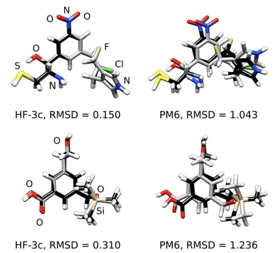
HF-3c is a lightweight Hartree–Fock method, using a minimal basis set derived from Huzinaga’s MINIS basis set. To ameliorate the issues that Hartree–Fock and a tiny basis set cause, the authors layer in three corrections: the D3 dispersion correction (with Becke–Johnson damping), their recent “gCP” geometric counterpoise correction for basis set incompleteness error, and an “SRB” short-range basis correction for electronegative elements.
HF-3c is surprisingly good at geometry optimization and noncovalent interaction energies (MAE of 0.39 kcal/mol on the S66 benchmark set), works okay for dipole moments and vibrational frequencies, but seems bad for anything involving bond breaking. Thus the authors recommend it for optimization of ground-state complexes, and not so much for finding an entire potential energy surface.
(One complaint about all of these papers: the basis set optimization isn’t described in much detail, and we basically have to take the authors’ word that what they came up with is actually the best.)
HF-3c(v) is pretty much the same as HF-3c, but it uses a “large-core” effective core potential to describe all of the core electrons, making it valence-only. This makes it 2–4 times faster, but also seems to make it much worse than HF-3c: I’m not sure the speed is worth the loss in accuracy.
The authors only use it to explore noncovalent interactions; I’m not sure if others have used it since.
PBEh-3c is the next “3c” method, and the first composite DFT method. As opposed to the minimal basis set employed in HF-3c, Grimme et al here elect to use a polarized double-zeta basis set, which “significantly improves the energetic description without sacrificing the computational efficiency too much.” They settle on a variant of def2-SV(P) with an effective core potential and a few other modifications, which they call “def-mSVP.”
As before, they also add the D3 and gCP corrections (both slightly modified), but they leave out the SRB correction. The biggest change is that they also reparameterize the PBE functional, which introduces an additional four parameters: three in PBE, and one to tune the percentage of Fock exchange. The authors note that increasing the Fock exchange from 25% to 42% offsets the error introduced by basis set incompleteness.
As before, the focus of the evaluation is on geometry optimization, and PBEh-3c seems to do very well (although not better than HF-3c on e.g. S66, which is surprising—the authors also don’t compare directly to HF-3c in the paper at all). PBEh-3c also does pretty well on the broad GMTKN30 database, which includes thermochemistry and barrier heights, faring just a bit worse than M06-2x/def2-SV(P).
HSE-3c is basically the same as PBEh-3c, but now using a screened exchange variant to make it more robust and faster for large systems or systems with small band gaps. The authors recommend using PBEh-3c for small molecules or large band-gap systems, which is my focus here, so I won’t discuss HSE-3c further.
B97-3c is another DFT composite method, but it’s a bit different than PBEh-3c. PBE is a pretty simple functional with only three tunable parameters, while B97 is significantly more complex with ten tunable parameters. Crucially, B97 is a pure functional, meaning that no Fock exchange is involved, which comes with benefits and tradeoffs. The authors write:
The main aim here is to complete our hierarchy of “3c” methods by approaching the accuracy of large basis set DFT with a physically sound and numerically well-behaved approach.
For a basis set, the authors use a modified form of def2-TZVP called “mTZVP”, arguing that “as the basis set is increased to triple-ζ quality, we can profit from a more flexible exchange correlation functional.” This time, the D3 and SRB corrections are employed, but the gCP correction is omitted.
The authors do a bunch of benchmarking: in general, B97-3c seems to be substantially better than either PBEh-3c or HF-3c at every task, which isn’t surprising given the larger basis set. B97-3c is also often better than e.g. B3LYP-D3 with a quadruple-zeta basis set, meaning that it can probably be used as a drop-in replacement for most routine tasks.
B3LYP-3c is a variant of PBEh-3c where you just remove the PBEh functional and replace it with B3LYP (without reparameterizing B3LYP at all). This is done to improve the accuracy for vibrational frequencies, since B3LYP performs quite well for frequencies. I’ve only seen this in one paper, so I’m not sure this will catch on (although it does seem to work).
Continuing our journey through the “Jacob’s ladder” of composite functionals, we arrive at r2 SCAN-3c, based on the meta-GGA r2 SCAN functional. No reparameterization of the base functional is performed, but the D4 and gCP corrections are added, and yet another basis set is developed: mTZVPP, a variant of the mTZVP basis set developed for B97-3c, which was already a variant of def2-TZVP.
The authors describe the performance of r2 SCAN-3c in rather breathless terms:
…we argue that r2 SCAN is the first mGGA functional that truly climbs up to the third rung of the Jacobs ladder without significant side effects (e.g., numerical instabilities or an overfitting behavior that leads to a bad performance for the mindless benchmark set).
…the new and thoroughly tested composite method r2 SCAN-3c provides benchmark-accuracy for key properties at a fraction of the cost of previously required hybrid/QZ approaches and is more robust than any other method of comparable cost. This drastically shifts the aforementioned balance between the computational efficiency and accuracy, enabling much larger and/or more thorough screenings and property calculations. In fact, the robustness and broad applicability of r2 SCAN-3c caused us to rethink the very structure of screening approaches.
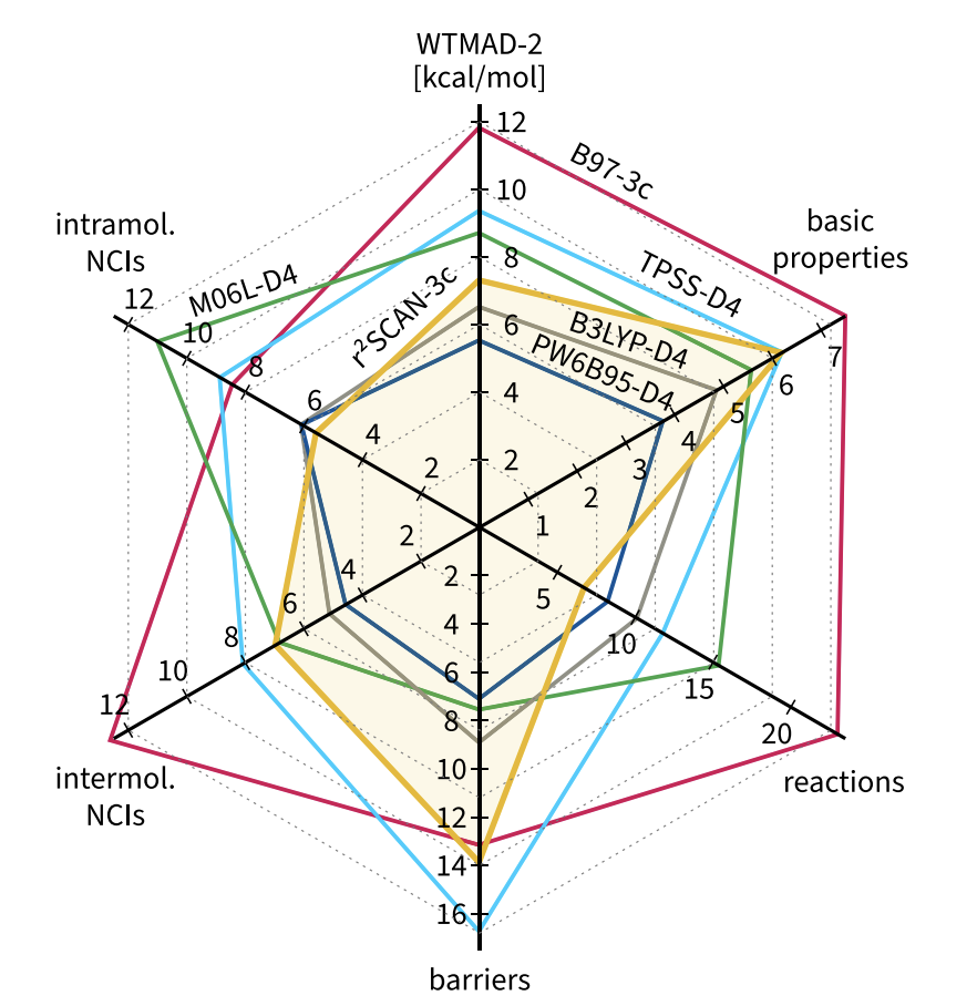
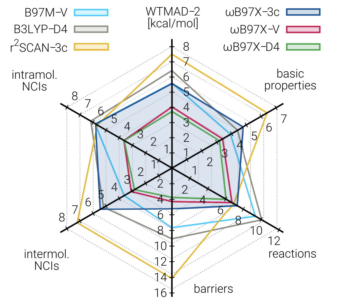
The amount of benchmarking performed is a little overwhelming. Here’s a nice figure that summarizes r2 SCAN-3c on the GMTKN55 database, and also compares it to B97-3c:
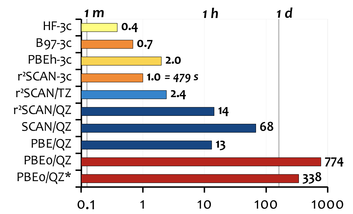
And here’s a nice graph that shows time comparisons for a 153-atom system, which is something that’s obviously a key part of the value-add:
Finally, we come to ωB97X-3c, a composite range-separated hybrid functional derived from Mardirossian and Head-Gordon’s ωB97X-V functional (which seems to me to be one of the best DFT methods, period). ωB97X-3c reintroduces Fock exchange, so it’s significantly more expensive than r2 SCAN-3c or B97-3c, but with this expense comes increased accuracy.
Interestingly, neither of the “weird” corrections (gCP or SRB) are employed for ωB97X-3c: it’s just an off-the-shelf unmodified functional, the now-standard D4 dispersion correction, and a specialized basis set. The authors acknowledge this:
Although ωB97X-3c is designed mostly in the spirit of the other “3c” methods, the meaning and definition of the applied “three corrections” have changed over the years. As before, the acronym stands for the dispersion correction and for the specially developed AO basis set, but here for the compilation of ECPs, which are essential for efficiency, as a third modification.
(But weren’t there ECPs before? Doesn’t even HF-3c have ECPs? Aren’t ECPs just part of the basis set? Just admit that this is a “2c” method, folks.)
The authors devote a lot of effort to basis-set optimization, because range-separated hybrids are so expensive that using a triple-zeta basis set like they did for B97-3c or r2 SCAN-3c would ruin the speed of the method. This time, they do go into more details, and emphasize that the basis set (“vDZP”) was optimized on molecules and not just on single atoms:
Molecule-optimized basis sets are rarely used in quantum chemistry. We are aware of the MOLOPT sets in the CP2K code and the polarization consistent (pc-n) basis sets by Jensen. In the latter, only the polarization functions are optimized with respect to molecular energies. A significant advantage of molecular basis set optimizations is that, contrary to atomic optimizations, all angular momentum functions (i.e., polarization functions not occupied in the atomic ground state) can be determined consistently, as already noted by VandeVondele and Hutter.
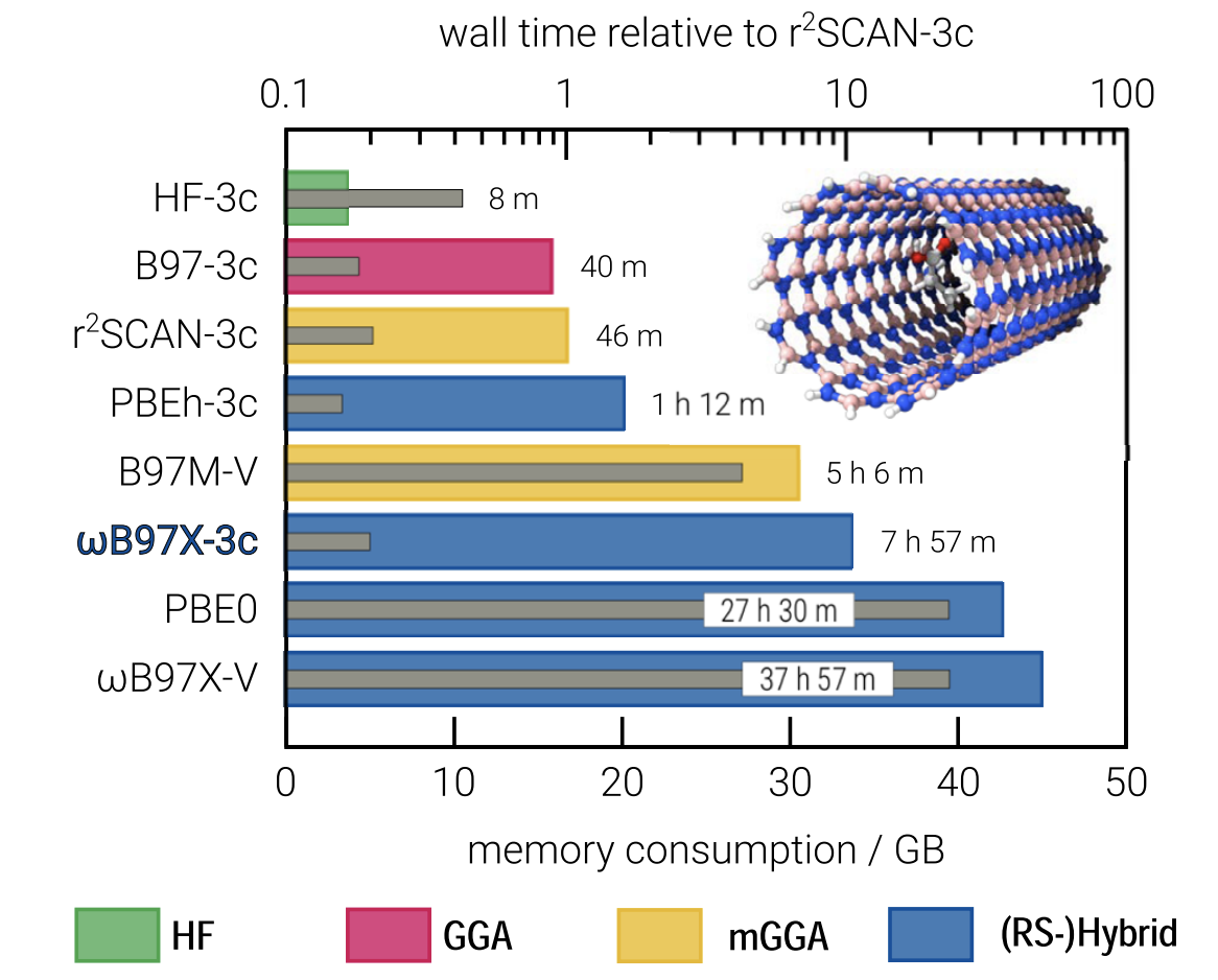
They also put together a new set of effective core potentials, which also helps to minimize the number of basis functions. Even so, ωB97X-3c is the slowest of the composite methods, as shown in this figure:
In terms of accuracy, ωB97X-3c is far better than r2 SCAN-3c, previously the best composite method, and is among the best-performing DFT methods in general for most benchmarks, although still outcompeted by ωB97X-V (and its close cousin ωB97X-D4, reparameterized in this work). The expense of ωB97X-3c means that for easy tasks like geometry optimization r2 SCAN-3c is still probably a better choice, but for almost anything else it seems that ωB97X-3c is an excellent choice.
An interesting observation is that ωB97X-3c is not just Pareto-optimal, but close to optimal in an absolute sense. I initially framed the goal of composite methods as finding new ways to increase speed while decreasing accuracy: but here it seems that we can gain a ton of speed without losing much accuracy at all! This should be somewhat surprising, and the implications will be discussed later.
Excluding some of the more specific composite methods, there seem to be three tiers here:
After decades of theorists mocking people for using small basis sets, it’s ironic that intentionally embracing cancellation of error is trendy again. I’m glad to see actual theorists turn their attention to this problem: people have never stopped using “inadequate” basis sets like 6-31G(d), simply because nothing larger is practical for many systems of interest!
The results from this body of work suggest that current basis sets are far from optimal, too. The only piece of ωB97X-3c that’s new is the basis set, and yet that seems to make a huge difference relative to state-of-the-art. What happens if vDZP is used for other methods, like B97? The authors suggest that it might be generally effective, but more work is needed to study this further.
Update: Jonathon Vandezande and I investigated this question, and it turns out vDZP is effective with other density functionals too. You can read our preprint here!
Basis-set optimization seems like a “schlep” that people have avoided because of how annoying it is, or something which is practically useful but not very scientifically interesting or publishable. Perhaps the success of composite methods will push more people towards studying basis sets; I think that would be a good outcome of this research. It seems unlikely to me that vDZP cannot be optimized further; if the results above are any indication, the Pareto frontier of basis sets can be advanced much more.
I’m also curious if Grimme and friends would change HF-3c and the other early methods, knowing what they know now. Do better basis sets alleviate the need for gCP and SRB, or is that not possible with a minimal basis set? What about D3 versus D4 (which wasn’t available at the time)? Hopefully someone finds the time to go back and do this, because to my knowledge HF-3c sees a good amount of use.
Perhaps my favorite part of this work, though, is the ways in which composite methods reduce the degrees of freedom available to end users. “Classic” DFT has a ton of tunable parameters (functional, basis set, corrections, solvent models, thresholds, and so forth), and people frequently make inefficient or nonsensical choices when faced with this complexity. In contrast, composite methods make principled and opinionated choices for many of these variables, thus giving scientists a well-defined menu of options.
This also makes it easier for outsiders to understand what’s going on. I wrote about this over a year ago:
While a seasoned expert can quickly assess the relative merits of BYLP/MIDI! and DSD-PBEP86/def2-TZVP, to the layperson it’s tough to guess which might be superior… The manifold diversity of parameters employed today is a sign of [computational chemistry]’s immaturity—in truly mature fields, there’s an accepted right way to do things.
The simplicity of composite methods cuts down on the amount of things that you have to memorize in order to understand computational chemistry. You only have to remember “HF-3c is fast and sloppy,” rather than trying to recall how many basis functions pcseg-1 has or which Minnesota functional is good for main-group geometries.
So, I’m really optimistic about this whole area of research, and I’m excited that other labs are now working on similar things (I didn’t have space to cover everyone’s contributions, but here’s counterpoise work from Head-Gordon and atom-centered potentials from DiLabio). The next challenge will be to get these methods into the hands of actual practitioners…