An important problem with simulating chemical reactions is that reactions generally take place in solvent, but most simulations are run without solvent molecules. This is a big deal, since much of the inaccuracy associated with simulation actually stems from poor treatment of solvation: when gas phase experimental data is compared to computations, the results are often quite good.
Why don’t computational chemists include solvent molecules in their models? It takes a lot of solvent molecules to accurately mimic bulk solvent (enough to cover the system with a few different layers, usually ~103).1 Since most quantum chemical methods scale in practice as O(N2)–O(N3), adding hundreds of additional atoms has a catastrophic effect on the speed of the simulation.
To make matters worse, the additional degrees of freedom introduced by the solvent molecules are very “flat”—solvent molecules don’t usually have well-defined positions about the substrate, meaning that the number of energetically accessible conformations goes to infinity (with attendant consequences for entropy). This necessitates a fundamental change in how calculations are performed: instead of finding well-defined extrema on the electronic potential energy surface (ground states or transition states), molecular dynamics (MD) or Monte Carlo simulations must be used to sample from an underlying distribution of structures and reconstruct the free energy surface. Sufficient sampling usually requires consideration of 104–106 individual structures,2 meaning that each individual computation must be very fast (which is challenging for quantum chemical methods).

Given the complexity this introduces, it’s not surprising that most computational organic chemists try to avoid explicit solvent at all costs. The typical workaround is to use “implicit solvent” models, which “reduce the complexity of individual solvent−solute interactions such as hydrogen-bond, dipole−dipole, and van der Waals interactions into a fictitious surface potential... scaled to reproduce the experimental solvation free energies” (Baik). This preserves the well-defined potential energy surfaces that organic chemists are accustomed to, so you can still find transition states by eigenvector following, etc.
Implicit solvent models like PCM, COSMO, or SMD are better than nothing, but are known to struggle for charged species. In particular, they don’t really describe explicit inner-sphere solvent–solute interactions (like hydrogen bonding), meaning that they’ll behave poorly when these interactions are important. Dan Singleton’s paper on the Baylis–Hillman reaction is a nice case study of how badly implicit solvent can fail: even high-level quantum chemical methods are useless when solvation free energies are 10 kcal/mol off from experiment!
This issue is well-known. To quote from Schreiner and Grimme:
An even more important but still open issue is solvation. In the opinion of the authors it is a ‘scandal’ that in 2018 no routine free energy solvation method is available beyond (moderately successful) continuum theories such as COSMO-RS and SMD and classical FF/MD-based explicit treatments.
When computational studies have been performed in explicit solvent, the results have often been promising: Singleton has studied diene hydrochlorination and nitration of toluene, and Peng Liu has recently conducted a nice study of chemical glycosylation. Nevertheless, these studies all require heroic levels of effort: quantum chemistry is still very slow, and so a single free energy surface might take months and months to compute.3
One promising workaround is using machine learning to accelerate quantum chemistry. Since these MD-type studies look at the same exact system over and over again, we could imagine first training some sort of ML model based on high-level quantum chemistry data, and then employing this model over and over again for the actual MD run. As long as (1) the ML model is faster than the QM method used to train it and (2) it takes less data to train the ML model than it would to run the simulation, this will save time: in most cases, a lot of time.
(This is a somewhat different use case than e.g. ANI-type models, which aim to achieve decent accuracy for any organic molecule. Here, we already know what system we want to study, and we’re willing to do some training up front.)
A lot of people are working in this field right now, but today I want to highlight some work that I liked from Fernanda Duarte and co-workers. Last year, they published a paper comparing a few different ML methods for studying quasiclassical dynamics (in the gas phase), and found that atomic cluster expansion (ACE) performed better than Gaussian approximation potentials while training faster than NequIP. They then went on to show that ACE models could be trained automatically through active learning, and used the models to successfully predict product ratios for cycloadditions with post-TS bifurcations.
Their new paper, posted on ChemRxiv yesterday, applies the same ACE/active learning approach to studying reactions in explicit solvent, with the reaction of cyclopentadiene and methyl vinyl ketone chosen as a model system. This is more challenging than their previous work, because the ML model now not only has to recapitulate the solute reactivity but also the solute–solvent and solvent–solvent interactions. To try and capture all the different interactions efficiently, the authors ended up using four different sets of training data: substrates only, substrates with 2 solvent molecules, substrates with 33 solvent molecules, and clusters of solvent only.
Previously, the authors used an energy-based selector to determine if a structure should be added to the training set: they predicted the energy with the model, ran a QM calculation, and selected the structure if the difference between the two values was big enough. This approach makes a lot of sense, but has the unfortunate downside that a lot of QM calculations are needed, which is exactly what this ML-based approach is trying to avoid. Here, the authors found that they could use similarity-based descriptors to select data points to add to the training set: these descriptors are both more efficient (needing fewer structures to converge) and faster to compute, making them overall a much better choice. (This approach is reminiscent of the metadynamics-based approach previously reported by John Parkhill and co-workers.)
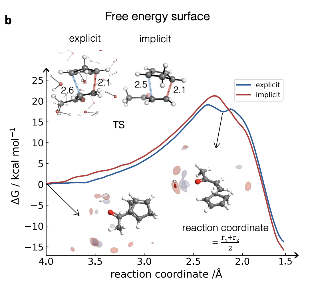
With a properly trained model in hand, the authors went on to study the reaction with biased sampling MD. They find that the reaction is indeed accelerated in explicit water, and that the free energy surface begins to look stepwise, as opposed to the concerted mechanism predicted in implicit solvent. (Singleton has observed similar behavior before, and I’ve seen this too.) They do some other interesting studies: they look at the difference between methanol and water as solvents, argue that Houk is wrong about the role of water in the TS,4 and suggest that the hydrophobic effect drives solvent-induced rate acceleration.5

The results they find for this particular system are interesting, but more exciting is the promise that these techniques may soon become accessible to “regular” computational chemists. Duarte and co-workers have shown that ML can be used to solve an age-old problem in chemical simulation; if explicit solvent ML/MD simulations of organic reactions become easy enough for non-experts to run, I have no doubt that they will become a valued and essential part of the physical organic chemistry toolbox. Much work is needed to get to that point—new software packages, further validation on new systems, new ways to assess quality and check robustness of simulations, and much more—but the vision behind this paper is powerful, and I can’t wait until it comes to fruition.
Thanks to Croix Laconsay for reading a draft of this post.