If you are a scientist, odds are you should be reading the literature more. This might not be true in every case—one can certainly imagine someone who reads the literature too much and never does any actual work—but as a heuristic, my experience has been that most people would benefit from reading more than they do, and often much more. Despite the somewhat aggressive title, my hope in writing this is to encourage you to read the literature more: to make you excited about reading the literature, not to guilt you into it or provoke anxiety.
Why You Should Read The Literature More
You should read the literature because you are a scientist, and your business is ideas. The literature is the vast, messy, primal chaos that contains centuries of scientific ideas. If you are an ideas worker, this is your raw material—this is what you work with. Not reading the literature as an ideas worker is like not going to new restaurants as a new chef, or not looking at other people’s art as an artist, or not listening to music as a composer. Maybe the rare person has an internal creativity so deep that they don’t need any external sources of inspiration, but I’m not sure I know anyone like that.
If you buy the concept of “domain arbitrage” I outlined last week, then reading the literature becomes doubly important for up-and-coming arbitrageurs. Not only do you need to stay on top of research in your own field, but you also need to keep an eye on other fields, to look for unexpected connections. It was only after months of reading physical chemistry papers about various IR spectroscopy techniques, with no direct goal in mind, that I realized I could use in situ IR to pin down the structure of ethereal HCl; simply reading organic chemistry papers would not have given me that insight.
How You Can Read The Literature More
If you don’t read the literature at all—like me, when I started undergrad—then you should start small. I usually recommend JACS to chemists. Just try to read every paper in your subfield in JACS for a few months; I began by trying to read every organic chemistry paper in JACS. At the beginning, probably only 10–20% will make sense. But if you push through and keep trying to make sense of things, eventually it will get easier. You’ll start to see the same experiments repeated, understand the structure of different types of papers, and even recognize certain turns of phrase. (This happened to me after about a year and a half of reading the literature.)
Reading more papers makes you a faster reader. Here’s Tyler Cowen on how he reads so quickly (not papers specifically, but still applicable):
The best way to read quickly is to read lots. And lots. And to have started a long time ago. Then maybe you know what is coming in the current book. Reading quickly is often, in a margin-relevant way, close to not reading much at all.
Note that when you add up the time costs of reading lots, quick readers don’t consume information as efficiently as you might think. They’ve chosen a path with high upfront costs and low marginal costs. "It took me 44 years to read this book" is not a bad answer to many questions about reading speed.
All of Tyler’s advice applies doubly to scientific writing, which is often jargon-filled and ordered in arcane ways. After 7ish years of reading the scientific literature, I can “skim” a JACS paper pretty quickly and determine what, if anything, is likely to be novel or interesting to me, which makes staying on top of the literature much easier than it used to be.
Once you are good with a single journal, you can expand to multiple journals. A good starting set for organic chemistry is JACS, Science, Nature, Nature Chemistry, and Angewandte. If you already know how to read papers quickly, it will not be very hard to read more and more papers. But expanding to new journals brings challenges: how do you keep up with all of them at once? Lots of people use an RSS feed to aggregate different journals—I use Feedly, as do several of my coworkers. (You can also get this blog on Feedly!)
I typically check Feedly many times a day on my phone; I can look at the TOC graphic, the abstract, and the title, and then if I like how the paper looks I’ll email it to myself. Every other day or so, I sit down at my computer with a cup of coffee and read through the papers I’ve emailed to myself. This is separate from my “pursuing ideas from my research”/”doing a literature dive for group meeting” way of reading the literature—this is just to keep up with all the cool stuff that I wouldn’t otherwise hear about.
“Inbox Zero” often proves elusive.
(I also use Google Scholar Alerts to email me when new labs publish results—I have probably 20-30 labs set up this way, just to make sure I don’t miss results that might be important just because they’re not in a high-profile journal.)
Keeping track of papers you actually like and want to remember is another challenge. For the past two years, I’ve put the URLs into a Google Sheet, along with a one-sentence summary of the paper, which helps me look through my “most liked” papers when I want to find something. Sadly, I didn’t do this earlier, so I’m often tormented by papers I dimly remember but can no longer locate.
What Literature You Should Read
This obviously depends on what you’re doing, but I tend to think about literature results in three categories:
Things every scientist should know about
Things I am supposed to be an expert on
Things I’m not supposed to be an expert on, but would still like to know about
Category 1 basically covers the highest profile results (Science and Nature), and these days Twitter makes that pretty easy.
Category 2 covers things “in-field” or directly related to my projects—anything it would be somewhat embarrassing not to know about. For me, this means JACS, Angewandte, ACS Catalysis, Org. Lett., OPRD, Organometallics, J. Org. Chem., and Chem. Sci. (I also follow Chem. Rev. and Chem. Soc. Rev., because review articles are nice.)
Category 3 covers things that I am excited to learn about. Right now, that’s JCTC and J. Phys. Chem. A–C. In the past, that’s included ACS Chem. Bio., Nature Chem. Bio., and Inorganic Chemistry. (Writing this piece made me realize I should follow JCIM and J. Chem. Phys., so I just added them to Feedly.)
Conclusion
Reading the literature is—in the short term—pointless, sometimes frustrating, and just a waste of time. It’s rare that the article you read today will lead to an insight on the problem you’re currently facing! But the gains to knowledge compound over time, so spending time reading the literature today will make you a much better scientist in the long run.
Thanks to Ari Wagen and Joe Gair for reading drafts of this post.
It’s a truth well-established that interdisciplinary research is good, and we all should be doing more of it (e.g. this NSF page). I’ve always found this to be a bit uninspiring, though. “Interdisciplinary research” brings to mind a fashion collaboration, where the project is going to end up being some strange chimera, with goals and methods taken at random from two unrelated fields.
Rather, I prefer the idea of “domain arbitrage.”1 Arbitrage, in economics, is taking advantage of price differences in different markets: if bread costs $7 in Cambridge but $4 in Boston, I can buy in Boston, sell in Cambridge, and pocket the difference. Since this is easy and requires very little from the arbitrageur, physical markets typically lack opportunities for substantial arbitrage. In this case, the efficient market hypothesis works well.
Knowledge markets, however, are much less efficient than physical markets—many skills which are cheap in a certain domain are expensive in other domains. For instance, fields that employ organic synthesis, like chemical biology or polymer chemistry, have much less synthetic expertise than actual organic synthesis groups. The knowledge of how to use a Schlenk line properly is cheap within organic chemistry but expensive everywhere else. And organic chemists certainly don’t have a monopoly on scarce skills: trained computer scientists are very scarce in most scientific fields, as are statisticians, despite the growing importance of software and statistics to almost every area of research.
Domain arbitrage, then, is taking knowledge that’s cheap in one domain to a domain where it’s expensive, and profiting from the difference. I like this term better because it doesn’t imply that the goal of the research has to be interdisciplinary—instead, you’re solving problems that people have always wanted to solve, just now with innovative methods. And the concept of arbitrage highlights how this can be beneficial for the practitioner. You’re bringing new insights to your field so you can help your own research and make cool discoveries, not because you’ve been told that interdisciplinary work is good in an abstract way.
There are many examples of domain arbitrage,2 but perhaps my favorite is the recent black hole image, which was largely due to work by Katie Bouman (formerly a graduate student at MIT, now a professor at Caltech):
The black hole picture, extracted from noisy radio telescope data by Bouman’s new algorithms.
What’s surprising is that Bouman didn’t have a background in astronomy at all: she “hardly knew what a black hole was” (in her words) when she started working on the project. Instead, Bouman’s work drew on her background in computer vision, adapting statistical image models to the task of reconstructing astronomical images. In a 2016 paper, she explicitly credits computer vision with the insights that would later lead to the black hole image, and concludes by stating that “astronomical imaging will benefit from the crossfertilization of ideas with the computer vision community.”
If we accept that domain arbitrage is important, why doesn’t it happen more often? I can think of a few reasons: some fundamental, some structural, and some cultural. On the fundamental level, domain arbitrage requires knowledge of two fields of research at a more-than-superficial level. This is relatively common for adjacent fields of research (like organic chemistry and inorganic chemistry), but becomes increasingly rare as the distance between the two fields grows. It’s not enough to just try and read journals from other fields occasionally—without the proper context, other fields are simply unintelligible. Given how hard achieving competence in a single area of study can be, we should not be surprised that those with a working knowledge of multiple fields are so scarce.
The structure of our research institutions also makes domain arbitrage harder. In theory, a 15-person research group could house scientists from a variety of backgrounds: chemists, biologists, mathematicians, engineers, and so forth, all focused on a common research goal. In practice, the high rate of turnover in academic positions makes this challenging. Graduate students are only around for 5–6 years, postdocs for fewer, and both positions are typically filled by people hoping to learn things, not by already competent researchers. Thus, senior lab members must constantly train newer members in various techniques, skills, and ways of thinking so that institutional knowledge can be preserved.
This is hard but doable for a single area of research, but quickly becomes untenable as the number of fields increases. A lab working in two fields has to pass down twice as much knowledge, with the same rate of personnel turnover. In practice, this often means that students end up deficient in one (or both) fields. As Derek Lowe put it when discussing chemical biology in 2007:
I find a lot of [chemical biology] very interesting (though not invariably), and some of it looks like it could lead to useful and important things. My worry, though, is: what happens to the grad students who do this stuff? They run the risk of spending too much time on biology to be completely competent chemists, and vice versa.
To me, this seems like a case in which the two goals of the research university—to teach students and to produce research—are at odds. It’s easier to teach students in single-domain labs, but the research that comes from multiple domains is superior. It’s not easy to think about how to address this without fundamental change to the structure of universities (although perhaps others have more creative proposals than I).3
But, perhaps most frustratingly, cultural factors also contribute to the rarity of domain arbitrage. Many scientific disciplines today define themselves not by the questions they’re trying to solve but by the methods they employ, which disincentivizes developing innovative methods. For example, many organic chemists feel that biocatalysis shouldn’t be considered organic synthesis, since it employs enzymes and cofactors instead of more traditional catalysts and reagents, even though organic synthesis and biocatalysis both address the same goal: making molecules. While it’s somewhat inevitable that years of lab work leaves one with a certain affection for the methods one employs, it’s also irrational.
Now, one might reasonably argue that precisely delimiting where one scientific field begins and another ends is a pointless exercise. Who’s to say whether biocatalysis is better viewed as the domain of organic chemistry or biochemistry? While this is fair, it’s also true that the scientific field one formally belongs to matters a great deal. If society deems me an organic chemist, then overwhelmingly it is other organic chemists who will decide if I get a PhD, if I obtain tenure as a professor, and if my proposals are funded.4
Given that the success or failure of my scientific career thus depends on the opinion of other organic chemists, it starts to become apparent why domain arbitrage is difficult. If I attempt to solve problems in organic chemistry by introducing techniques from another field, it’s likely that my peers will be confused or skeptical by my work, and hesitate to accept it as “real” organic chemistry (see, for instance, the biocatalysis scenario above). Conversely, if I attempt to solve problems in other domains with the tools of organic chemistry, my peers will likely be uninterested in the outcome of the research, even if they approve of the methods employed. So from either angle domain arbitrage is disfavored.
The factors discussed here don’t serve to completely halt domain arbitrage, as successful arbitrageurs like Katie Bouman or Frances Arnold demonstrate, but they do act to inhibit it. If we accept the claim that domain arbitrage is good, and we should be working to make it more common, what then should we do to address these problems? One could envision a number of structural solutions, which I won’t get into here, but on a personal level the conclusion is obvious: if you care about performing cutting-edge research, it’s important to learn things outside the narrow area that you specialize in and not silo yourself within a single discipline.
Thanks to Shlomo Klapper and Darren Zhu for helpful discussions. Thanks also to Ari Wagen, Eric Gilliam, and Joe Gair for editing drafts of this post; in particular, Eric Gilliam pointed out the cultural factors discussed in the conclusion of the post.
Footnotes
I did not coin this term—credit goes to Shlomo Klapper. I do think this is the first time it's been used in writing, however.
I'll actually go a step farther and propose the Strong Theorem of Domain Arbitrage: All non-incremental scientific discoveries arise either from domain arbitrage or random chance. I don't want to defend it here, but I think there's a reasonable chance that this is true.
Collaborations between differently skilled labs help with this problem, but the logistical and practical challenges involved in collaboration make this an inefficient solution. Plus, the same cultural challenges still confront the individual contributors.
Recently, I’ve been working to assign the relative configuration of some tricky diastereomers, which has led me to do a bit of a deep dive into the world of computational NMR prediction. Having spent the last week or so researching the current state-of-the-art in simulating experimental 1H NMR spectra, I’m excited to share some of my findings.
My main resource in this quest has been a new NMR benchmarking paper, published on March 7th by authors from Merck (and a few other places). Why this paper in particular? Although there have been many NMR benchmarks, not all of these papers are as useful as they seem. Broadly speaking, there are two ways to benchmark NMR shifts: (1) against high-level computed results or (2) against experimental NMR shifts.
The first strategy seems to be popular with theoretical chemists: NMR shifts at a very high level of theory are presumably very accurate, and so if we can just reproduce those values with a cheap method, we will have solved the NMR prediction problem. Of course, effects due to solvation and vibrational motion will be ignored, but these effects can always be corrected for later. In contrast, the second strategy is more useful for experimental chemists: if the calculation is going to be compared to experimental NMR spectra in CDCl3 solution, the match with experiment is much more important than the gas-phase accuracy of the functional employed.
Not only are these two approaches different in theory, they yield vastly different results in practice, as is nicely illustrated by the case of the double-hybrid functional DSD-PBEP86. DSD-PBEP86 was first reported in 2018 by Frank Neese and coworkers, who found it to be much superior to regular DFT methods or MP2-type wavefunction methods at reproducing CCSD(T) reference data.1A subsequent benchmark by Kaupp and coworkers looked at a much larger set of compounds and confirmed that DSD-PBEP86 was indeed superior at reproducing CCSD(T) data, with a mean absolute error (MAE) for 1H of 0.06 ppm. In contrast, de Oliveira and coworkers found that DSD-PBEP86 and related double-hybrid methods were much worse at predicting experimental 1H NMR shifts, with a MAE of 0.20 ppm, making them no better than conventional DFT approaches.
The difference between these two mindsets is nicely demonstrated by Kaupp’s paper, which dismisses de Oliveira’s work as suffering from “methodological inadequacies” and states:
[Benchmarking] can be done by comparing approximative calculations to experimental data or to data computed using high-level ab initio methodologies. The latter helps to eliminate a number of factors that often complicate the direct comparison against experiment, such as environmental, ro-vibrational, or thermal contributions (possibly also relativistic effects, see below).
While Kaupp is correct that using gas-phase CCSD(T) data does eliminate “environmental” effects (e.g. from solvent), it’s not clear that these effects always ought to be eliminated! Although directly optimizing a computational method to reproduce a bunch of ill-defined environmental effects is perhaps inelegant, it’s certainly pragmatic.
The authors of the 2023 benchmark create a new set of well-behaved reference compounds that avoid troublesome heavy-atom effects (poorly handled by most conventional calculations) or low-lying conformational equilibria, and re-acquire experimental spectra (in chloroform) for every compound in the set. They then score a wide variety of computational methods against this dataset: functionals, basis sets, implicit solvent methods, and more.
In the end, Cramer’s WP04 functional is found to be best, which is perhaps unsurprising given that it was specifically optimized for the prediction of 1H shifts in chloroform.2 The WP04/6-311++G(2d,p)/PCM(chloroform) level of theory is optima, giving an MAE of 0.08 ppm against experiment, but WP04/jul-CC-PVDZ/PCM(chloroform) is cheaper and not much worse. B3LYP-D3/6-31G(d) works fine for geometry optimization, as do wB97X-D/6-31G(d) and M06-2X/6-31G(d).
Based on these results, my final workflow for predicting experimental proton spectra is:
Optimize each conformer using B3LYP-D3BJ/6-31G(d).
Remove duplicate conformers with cctk.ConformationalEnsemble.eliminate_redundant().
Predict NMR shifts for each conformer using WP04/6-311++G(2d,p)/PCM(chloroform).
Combine conformer predictions through Boltzmann weighting, and apply a linear correction.
For small molecules, this workflow runs extremely quickly (just a few hours from start to finish), and has produced good-quality results that solved the problem I was trying to solve.
Nevertheless, the theoreticians have a point—although WP04 can account for a lot of environmental effects (essentially by overfitting to experimental data), there are plenty of systems for which this pragmatic approach cannot succeed. For instance, the DELTA50 dataset intentionally excludes molecules which might exhibit concentration-dependent aggregation behavior, which includes basically anything capable of hydrogen bonding or π–π stacking! If we hope to get beyond a certain level of accuracy, it seems likely that physically correct models of NMR shieldings, solvent effects, and aggregation will be necessary.
The WP04 functional is not technically in Gaussian, but can be employed with the following route card: #p nmr=giao BLYP IOp(3/ 76=1000001189,3/77=0961409999,3/78=0000109999) 6-311++G(2d,p) scrf=(pcm,solvent=chloroform).
Python is an easy language to write, but it’s also veryslow. Since it’s a dynamically typed and interpreted language, every Python operation is much slower than the corresponding operation would be in C or FORTRAN—every line of Python must be interpreted, type checked, and so forth (see this little overview of what the Python interpreter does).
Fortunately for those of us who like programming in Python, there are a number of different ways to make Python code faster. The simplest way is just to use NumPy, the de facto standard for any sort of array-based computation in Python; NumPy functions are written in C/C++, and so are much faster than the corresponding native Python functions.
Another strategy is to use a just-in-time compiler to accelerate Python code, like Jax or Numba. This approach incurs a substantial O(1) cost (compilation) but makes all subsequent calls orders of magnitude faster. Unfortunately, these libraries don’t support all possible Python functions or external libraries, meaning that sometimes it’s difficult to write JIT-compilable code.
How do these strategies fare on a real-world problem? I selected pairwise distance calculations for a list of points as a test case; this problem is pretty common in a lot of scientific contexts, including calculating electrostatic interactions in molecular dynamics or quantum mechanics.
We can start by importing the necessary libraries and writing two functions. The first function is the “naïve” Python approach, and the second uses scipy.spatial.distance.cdist, one of the most overpowered functions I’ve encountered in any Python library.
import numpy as np
import numba
import cctk
import scipy

mol = cctk.XYZFile.read_file("30_dcm.xyz").get_molecule()
points = mol.geometry.view(np.ndarray)

def naive_get_distance(points):
    N = points.shape[0]
    distances = np.zeros(shape=(N,N))
    for i, A in enumerate(points):
        for j, B in enumerate(points):
            distances[i,j] = np.linalg.norm(A-B)
    return distances

def scipy_get_distance(points):
    return scipy.spatial.distance.cdist(points,points)
If we score these functions in Jupyter, we can see that cdist is almost 2000 times faster than the pure Python function!
%%timeit
naive_get_distance(points)

103 ms ± 981 µs per loop (mean ± std. dev. of 7 runs, 10 loops each)
%%timeit
scipy_get_distance(points)

55.2 µs ± 2.57 µs per loop (mean ± std. dev. of 7 runs, 10000 loops each)
In this case, it’s pretty obvious that we should just use cdist. But what if there wasn’t a magic built-in function for this task—how close can we get to the performance of cdist with other performance optimizations?
The first and most obvious optimization is simply to take advantage of the symmetry of the matrix, and not compute entries below the diagonal. (Note that this is sort of cheating, since cdist doesn’t know that both arguments are the same.)
def triangle_get_distance(points):
    N = points.shape[0]
    distances = np.zeros(shape=(N,N))
    for i in range(N):
        for j in range(i,N):
            distances[i,j] = np.linalg.norm(points[i]-points[j])
            distances[j,i] = distances[i,j]
    return distances
As expected, this roughly halves our time:
%%timeit
triangle_get_distance(points)

57.6 ms ± 409 µs per loop (mean ± std. dev. of 7 runs, 10 loops each)
Next, we can use Numba to compile this function. This yields roughly a 10-fold speedup, bringing us to about two orders of magnitude slower than cdist.
%%timeit
numba_triangle_get_distance(points)

5.74 ms ± 36.2 µs per loop (mean ± std. dev. of 7 runs, 100 loops each)
Defining our own norm with Numba, instead of using np.linalg.norm, gives us another nice boost:
def custom_norm(AB):
    return np.sqrt(AB[0]*AB[0] + AB[1]*AB[1] + AB[2]*AB[2])

numba_custom_norm = numba.njit(custom_norm)

def cn_triangle_get_distance(points):
    N = points.shape[0]
    distances = np.zeros(shape=(N,N))
    for i in range(N):
        for j in range(i,N):
            distances[i,j] = numba_custom_norm(points[i] - points[j])
            distances[j,i] = distances[i,j]
    return distances

numba_cn_triangle_get_distance = numba.njit(cn_triangle_get_distance)
%%timeit
numba_cn_triangle_get_distance(points)

1.35 ms ± 21.6 µs per loop (mean ± std. dev. of 7 runs, 1000 loops each)
What about trying to write this program using only vectorized NumPy functions? This takes a bit more creativity; I came up with the following function, which is a bit memory-inefficient but still runs quite quickly:
def numpy_get_distance(points):
    N = points.shape[0]

    points_row = np.repeat(np.expand_dims(points,1), N, axis=1)
    points_col = np.repeat(np.expand_dims(points,0), N, axis=0)

    sq_diff = np.square(np.subtract(points_row, points_col))
    return np.sqrt(np.sum(sq_diff, axis=2))
%%timeit
numpy_get_distance(points)

426 µs ± 6.34 µs per loop (mean ± std. dev. of 7 runs, 1000 loops each)
Unfortunately, calling np.repeat with arguments isn’t supported by Numba, meaning that I had to get a bit more creative to write a Numba-compilable version of the previous program. The best solution that I found involved a few array reshaping operations, which are (presumably) pretty inefficient, and the final code only runs a little bit faster than the Numpy-only version.
%%timeit
numba_np_get_distance2(points)

338 µs ± 4.11 µs per loop (mean ± std. dev. of 7 runs, 1000 loops each)
I tried a few other approaches, but ultimately wasn’t able to find anything better; in theory, splitting the loops into chunks could improve cache utilization, but in practice anything clever I tried just made things slower.
In the end, we were able to accelerate our code about 250x by using a combination of NumPy and Numba, but were unable to match the speed of an optimized low-level implementation. Maybe in a future post I’ll drop into C or C++ and see how close I can get to the reference—until then, I hope you found this useful.
(I’m sure that there are ways that even this Python version could be improved; I did not even look at any other libraries, like Jax, Cython, or PyPy. Let me know if you think of anything clever!)
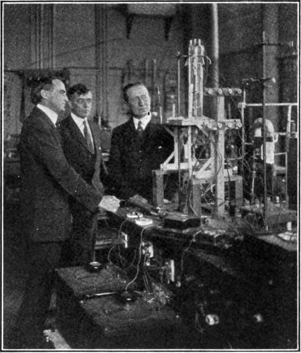
Eric Gilliam, whose work on the history of MIT I highlighted before, has a nice piece looking at Irving Langmuir’s time at the General Electric Research Laboratory and how applied science can lead to advances in basic research.
Gilliam recounts how Langmuir started working on a question of incredible economic significance to GE—how to make lightbulbs last longer without burning out—and after embarking on a years-long study of high-temperature metals under vacuum, not only managed to solve the lightbulb problem (by adding an inert gas to decrease evaporation and coiling the filament to prevent heat loss), but also starting working on the problems he would later become famous for studying. In Langmuir’s own words:
The work with tungsten filaments and gases done prior to 1915 [at the GE laboratory] had led me to recognize the importance of single layers of atoms on the surface of tungsten filaments in determining the properties of these filaments.
Indeed, Langmuir was awarded the 1932 Nobel Prize in Chemistry “for his discoveries and investigations in surface chemistry.”
Langmuir in the GE Research Laboratory.
Nor were lightbulbs the only thing Langmuir studied at GE: he invented a greatly improved form of vacuum pump, invented a hydrogen welding process used to construct vacuum-tight seals, and employed thin films of molecules on water to determine accurate molecular sizes with unprecedented accuracy. Gilliam argues that this tremendous productivity can in part be attributed to the fact that Langmuir’s work was in constant contact with practical problems, which served as a source of scientific inspiration:
In a developed world that is not exactly beset by scarcity and hardship anymore, it is hard to come up with the best areas to explore out of thin air. Pain points are not often obvious. Fundamental researchers can benefit massively from going to a lab mostly dedicated to making practical improvements to things like light bulbs and pumps and observing/asking questions. It is, frankly, odd that we normalized a system in which so many of our fundamental STEM researchers are allowed to grow so disjoint from the applied aspects of their field in the first place.
As [the GE] laboratory developed it was soon recognized that it was not practicable nor desirable that such a laboratory should be engaged wholly in fundamental scientific research. It was found that at least 75 per cent of the laboratory must be devoted to the development of the practical applications. It is stimulating to the men engaged in fundamental science to be in contact with those primarily interested in the practical applications.
Let’s bring in our second thinker. Last weekend, I had the privilege of attending a lecture by Johnathan Bi on Rene Girard and the philosophy of innovation, which discussed (among other things) how a desire for “disruption” above all else actually makes innovation more difficult. To quote Girard’s “Innovation and Repetition,” which Bi discussed at length:
The main prerequisite for real innovation is a minimal respect for the past and the mastery of its achievements, i.e., mimesis. To expect novelty to cleanse itself of imitation is to expect a plant to grow with its roots up in the air. In the long run, the obligation always to rebel may be more destructive of novelty than the obligation never to rebel.
What does this mean? Girard is describing two ways in which innovation can fail. The first is quite intuitive—if we hew to tradition too much, if we have an excessive respect for the past and not a “minimal respect,” we’ll be afraid to innovate. This is the oft-derided state of stagnation.
The second way in which we can fail to innovate, however, is a bit more subtle. Girard is saying that innovation also requires a mastery of the past’s achievements; we can’t simply ignore tradition, we have to understand what exists before we can innovate on top of it. Otherwise we will be, in Girard’s words, like a plant “with its roots up in the air.” All innovation has to occur within its proper context—to quote Tyler Cowen, “context is that which is scarce.”
This might seem a little silly. Innovation, “the introduction of new things, ideas or ways of doing something” (Oxford), at first inspection seems not to depend on tradition at all. But novelty with no hope of improvement over the status quo is simply a cry for attention; wearing one’s shoes on the wrong feet may be unusual, but is unlikely to win one renown as a great innovator.
When innovation, devoid of context, becomes the highest virtue... (I added this to the post a few hours late, sorry.)
What does this mean for scientific innovation, and how does this connect to Gilliam’s thoughts about Langmuir and the GE Research Laboratory? I’d argue that much of our fundamental research today, even that which is novel, lacks the context necessary to be transformatively innovative. Often the most impactful discoveries aren’t those which self-consciously aim to be Science or Nature papers, but those which simply aim to address outstanding problems or investigate anomalies. For instance, our own lab’s interest in hydrogen-bond-donor organocatalysis was initiated by the unexpected discovery that omitting the metal from an ostensibly metal-catalyzed Strecker reaction increased the enantioselectivity. Girard again:
The principle of originality at all costs leads to paralysis. The more we celebrate "creative and enriching" innovations, the fewer of them there are.
Langmuir’s example shows us a different path towards innovation. If we set out to investigate and address real-world problems of known practical import, without innovation in mind, Gilliam and Girard argue that we’ll be more innovative than if we make innovation our explicit goal. I don’t have a concrete policy recommendation to share here, but some of my other blog posts on applied research at MIT and the importance of engineering perhaps hint at what positive change might look like.
In accordance with the themes of this piece, my interpretation of Girard pretty much comes straight from Johnathan Bi. He has a lecture on Youtube where he discusses these ideas: here’s a link to the relevant segment, which is the only part I’ve watched.