An (in)famous code challenge in computer graphics is to write a complete ray tracer small enough to fit onto a business card. I've really enjoyed reading through some of the submissions over the years (e.g. 1, 2, 3, 4), and I've wondered what a chemistry-specific equivalent might be.
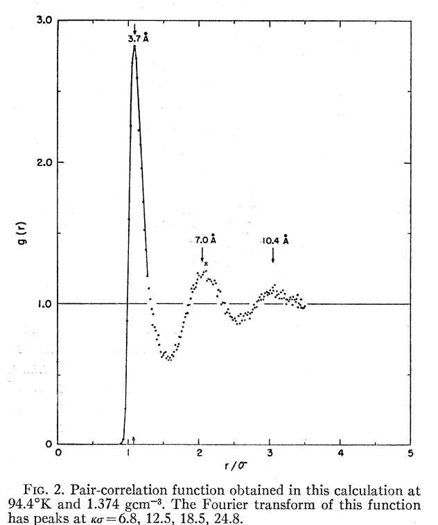
As a first step in this space—and as a learning exercise for myself as I try to learn C++—I decided to try and write a tiny Lennard–Jones simulation. Unlike most molecular simulation methods, which rely on heavily parameterized forcefields or complex quantum chemistry algorithms, the Lennard–Jones potential has a simple functional form and accurately models noble gas systems. Nice work from Rahman in 1964 showed that Lennard–Jones simulations of liquid argon could reproduce experimental X-ray scattering results for the radial distribution function:
This thus seemed like a good target for a "tiny chemistry" program: easy enough to be doable, but tricky enough to be interesting. After a bit of development, I was able to get my final program down to 1561 characters, easily small enough for a business card. The final program implements periodic boundary conditions, random initialization, and temperature control with the Berendsen thermostat for the first 10 picoseconds. Neighbor lists are used to reduce the computational cost, and an xyz file is written to stdout.
#include <iostream>
#include <random>
#define H return
typedef double d;typedef int i;using namespace std;d L=17;i N=860;d B=8.314e-7;d
 s=3.4;d M=6*s*s;d S=s*s*s*s*s*s;d q(d x){if(x>L)x-=2*L;if(x<-L)x+=2*L;H x;}d rd
(){H 2*L*drand48()-L;}struct v{d x,y,z;v(d a=0,d b=0,d c=0):x(a),y(b),z(c){}d n(
){H x*x+y*y+z*z;}v p(){x=q(x);y=q(y);z=q(z);H*this;}};v operator+(v a,v b){H v(a
.x+b.x,a.y+b.y,a.z+b.z);}v operator*(d a,v b){H v(a*b.x,a*b.y,a*b.z);}struct p{d
 m;v r,q,a,b;vector<i> W;p(v l,d n=40):r(l),m(n),q(v()),a(v()),b(v()),W(vector<i
>()){}void F(v f){b=(1/m)*f+b;}};vector<p> P;void w(){cout<<N<<"\n\n";for(i j=N;
j--;){v l=P[j].r;cout<<"Ar "<<l.x<<" "<<l.y<<" "<<l.z<<"\n";}cout<<"\n";}void E(
){for(i j=0;j<N;j++){for(i x=0;x<P[j].W.size();x++){i k=P[j].W[x];v R=(P[j].r+-1
*P[k].r).p();d r2=R.n();if(r2<M){d O=1/(r2*r2*r2);d f=2880*B*(2*S*S*O*O-S*O)/r2;
R=f*R;P[j].F(R);P[k].F(-1*R);}}}}void cW(){for(i j=0;j<N;j++){P[j].W.clear();for
(i k=j+1;k<N;k++)if((P[j].r+-1*P[k].r).p().n()<1.3*M)P[j].W.push_back(k);}}i mai
n(){i A=1e3;i e=75;i Y=5e3;for(i j=N;j--;){for(i a=99;a--;){v r=v(rd(),rd(),rd()
);i c=0;for(i k=P.size();k--;){d D=(r+-1*P[k].r).p().n();if(D<2*s)c=1;}if(!c){P.
push_back(p(r));break;}}}if(P.size()!=N)H 1;for(i t=0;t<=3e4;t+=10){for(i j=N;j-
-;){P[j].r=P[j].r+P[j].q+0.5*P[j].a;P[j].r.p();}if(t%20==0)cW();E();d K=0;for(i
j=N;j--;){P[j].q=P[j].q+0.5*(P[j].b+P[j].a);P[j].a=P[j].b;P[j].b=v();K+=P[j].m*P
[j].q.n()/2;}d T=2*K/(3*B*N);if(t<2*Y){d C=e;if(t<Y)C=e*t/Y+(A-e)*(Y-t)/Y;d s=sq
rt(C/T);for(i j=N;j--;)P[j].q=s*P[j].q;}if(t%100==0&&t>2*Y)w();}}
The program can be compiled with g++ -std=gnu++17 -O3 -o mini-md mini-md.cc and run:
$ time ./mini-md > Ar.xyz

real	0m4.689s
user	0m4.666s
sys	0m0.014s
Analysis of the resulting file in cctk results in the following radial distribution function, in good agreement with the literature:
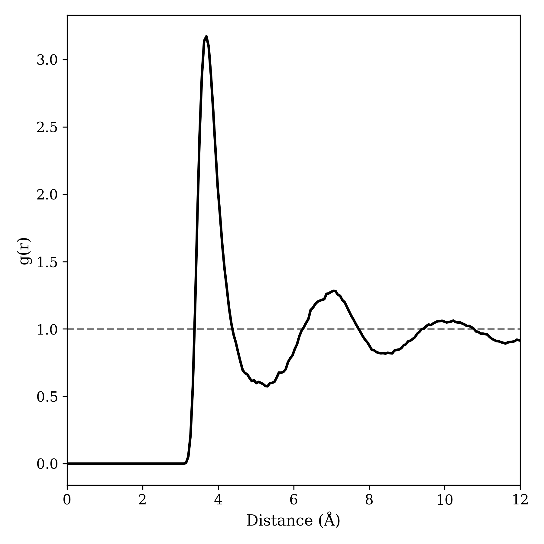
I'm pretty pleased with how this turned out, and I learned a good deal both about the details of C++ syntax and about molecular dynamics. There are probably ways to make this shorter or faster; if you write a better version, let me know and I'll happily link to it here!