Recently, I wrote about how scientists could stand to learn a lot from the tech industry. In that spirit, today I want to share a book review of Chaos Monkeys: Obscene Fortune and Random Failure in Silicon Valley, Antonio García Martínez’s best-selling memoir about his time in tech and “a guide to the spirit of Silicon Valley” (NYT).
Chaos Monkeys is one of the most literary memoirs I’ve read. The book itself is a clear homage to Hunter S. Thompson’s Fear and Loathing in Las Vegas; Martínez writes in the “gonzo journalism” style, blending larger-than-life personal exploits with frank accounting of the facts. But Antonio García Martínez’s writing, replete with GRE-level words and classical epigraphs, invites further literary comparisons.
Chaos Monkeys as The Odyssey
The first comparison that springs to mind is The Odyssey. Odysseus, the protagonist of The Odyssey, is frequently described as polytropos (lit. “many turns”), which denotes his wily and cunning nature. Antonio García Martínez (or, per the tech fondness for acronyms, “AGM”) certainly deserves the same epithet.
Chaos Monkeys is structured as a recounting of AGM’s escapades in Silicon Valley. In order, he (1) leaves his job at Goldman Sachs and joins an ad-tech company, (2) quits and founds his own company, AdGrok, (3) gets accepted to Y Combinator and survives a lengthy legal battle with his former employer, (4) sells AdGrok simultaneously to both Twitter and Facebook, eventually sending the other employees to Twitter and himself to Facebook, (5) becomes a PM at Facebook and engineers a scheme to fix their ad platform and make them profitable, (6) succeeds, sorta, but pisses people off and gets fired, and then (7) turns around and sells his expertise to Twitter.
His circuitous journey around the Bay Area has the rough form of an ancient epic: at each company, he’s faced with new challenges and new adversaries, and his fractious relationships with his superiors mean that he’s often at the mercy of capricious higher powers, not unlike Odysseus. Nevertheless, through a mixture of cunning and hard work he manages to escape with his skin intact every time, ready for the next episode. (And, best of all, he literally lives on a boat while working at Facebook.)
(His escapades have only continued since this book was published: he got hired at Apple, unceremoniously fired a few weeks later [for passages in Chaos Monkeys], made it on Joe Rogan, and has now founded spindl, a web3 ad-tech startup, while simultaneously converting to Judaism.)
Chaos Monkeys as Moby-Dick
Chaos Monkeys bears a structural resemblance to Moby-Dick. Narrative passages alternate with lengthy technical discussions about the minutiae of Silicon Valley: one chapter, you’re reading about how AGM flooded Mark Zuckerberg’s office trying to brew beer inside Facebook, while the next chapter is devoted to a discussion of how demand-side advertising platforms work.
The similarities run deeper, though. Venture capitalism, the funding model that dominates Silicon Valley, was originally developed to fund whaling expeditions in the 1800s (ref, ref). While once venture capitalists listened to prospective whaling captains advertising the quality of their crews in a New England tavern, today VCs hear pitches from thousands of startups hoping to develop the next killer app the best ChatGPT frontend and make millions.
This isn’t a coincidence: whaling expeditions and tech startups are both high-risk, high-reward enterprises that require an incredible amount of skill and hard work, but also a healthy dose of luck. Both operations have returns dominated by outliers, making picking winners much more important than making safe bets, and in both cases the investment remains illiquid for a long time, demanding trust from the investor.
Much like Ishmael in Moby-Dick, AGM’s adventures see him join forces with a motley crew of high-performing misfits from around the globe. And just as Ahab’s quest for the whale is foreshadowed to be a ruinous one, so too does the reader quickly come to understand that AGM’s tenure in Silicon Valley will not, ultimately, end well. A fatalistic haze hangs over the book, coloring his various hijinks with a sense of impending loss.
(And did I mention he lives on a boat?)
Chaos Monkeys as The Great Gatsby
The emotional tone of the book, however, is best compared to that favorite of high-school English classes, The Great Gatsby. AGM, like Nick Carraway, is an outsider in the world of the nouveau riche—opulent parties, high-speed road races, conspicuous consumption—and, over the course of the book, is alternately infatuated with and disgusted by his surroundings. When at last AGM retires to a quiet life on Ithaca the San Juan islands, it’s with feelings of disillusionment, betrayal, and frustration, not unlike Carraway withdrawing to the Midwest. As AGM writes in the penultimate paragraph of Chaos Monkeys’s acknowledgements:
To Paul Graham, Jessica Livingston, Sam Altman, and the rest of the Y Combinator partners and founders involved in the AdGrok saga. In a Valley world awash with mammoth greed and opportunism masquerading as beneficent innovation, you were the only real loyalty and idealism I ever encountered.
But Chaos Monkeys isn’t solely an indictment of Silicon Valley’s worst excesses. Not unlike The Wire, Chaos Monkeys manages to simultaneously portray the positive and negative aspects of its subject matter, refusing to be reduced to “tech good” or “tech bad.” The panoply of grifters, Dilbert-tier bosses, and Machiavellian sociopaths lambasted by AGM can exist only because of the immense value that their enterprises provide to society—and his faith in the ability of tech to create wonders persists even as his own efforts to do so are undermined.
So the underlying message of Chaos Monkeys, ultimately, is one of hope for tech. If the excesses of tech are worse than other industries, it's only because the underlying field itself is so much more fertile. Far from condemning it, the depths of the decadence spawned by Silicon Valley bear witness to the immense value it creates. Imitation is the highest form of flattery; grift is the surest sign of productivity.
Overall, Chaos Monkeys is an exhilarating and hilarious read, a gentle introduction to the world of term sheets, product managers, and non-competes, and a book replete with anecdotes sure to fulfill the stereotypes of tech-lovers and tech-haters alike.
Previously, I wrote about various potential future roles for journals. Several of the scenarios I discussed involved journals taking a much bigger role as editors and custodians of science, using their power to shape the way that science is conducted and exerting control over the scientific process.
I was thus intrigued when, last week, The Journal of Chemical Information and Modeling (JCIM; an ACS journal) released a set of guidelines for molecular dynamics simulations that future publications must comply with. These guidelines provoked a reaction from the community: various provisions (like the requirement that all simulations be performed in triplicate) were alleged to be arbitrary or unscientific, and the fact that these standards were imposed by editors and not determined by the community also drew criticism.
The authors say that the editorial “is *not* intended to instruct on how to run MD”, but this defense rings hollow to me. See, for instance, the section about choosing force fields:
JCIM will not accept simulations with old force field versions unless a clear justification is provided. Specialized force fields should be used when available (e.g., for intrinsically disordered proteins). In the case of the reparametrization or development of new parameters compatible with a given force field, please provide benchmark data to support the actual need for reparameterization, proper validation of novel parameters against experimental or high-level QM data…
I’m not a molecular dynamics expert, so I’m happy to stay out of the scientific side of things (although the editorial’s claim that “MD simulations are not suitable to sample events occurring between free energy barriers” seems clearly false for sufficiently low-barrier processes). Nor do I wish to overstate the size of the community’s reaction: a few people complaining on Twitter doesn’t really matter.
Rather, I want to use this vignette to reflect on the nature of scientific authority, and return to a piece I’ve cited before: Geoff Anders’ “The Transformations of Science.” Anders describes how the enterprise of science, initially intended to be free from authority, has evolved into a magisterium of knowledge that governments, corporations, and laypeople rely upon:
The original ideal of nullius in verba sometimes leads people to say that science is a never-ending exploration, never certain, and hence antithetical to claims on the basis of authority. This emphasizes one aspect of science, and indeed in theory any part of the scientific corpus could be overturned by further observations.
There is, however, another part of science—settled science. Settled science is safe to rely on, at least for now. Calling it into question should not be at the top of our priorities, and grant committees, for example, should typically not give money to researchers who want to question it again.
While each of these forms of science is fine on its own, they ought not to be conflated:
When scientists are meant to be authoritative, they’re supposed to know the answer. When they’re exploring, it’s okay if they don’t. Hence, encouraging scientists to reach authoritative conclusions prematurely may undermine their ability to explore—thereby yielding scientific slowdown. Such a dynamic may be difficult to detect, since the people who are supposed to detect it might themselves be wrapped up in a premature authoritative consensus.
This is tough, because scientists like settled science. We write grant applications describing how our research will bring clarity to long-misunderstood areas of reality, and fancy ourselves explorers of unknown intellectual realms. How disappointing, then, that so often science can only be relied upon when it settles, long after the original discoveries have been made! An intriguing experimental result might provoke further study, but it’s still “in beta” (to borrow the software expression) for years or decades, possibly even forever.
Applying the settled/unsettled framework of science to the JCIM question brings some clarity. I don’t think anyone would complain about settled science being used in editorial guidelines: I wouldn’t want to open JACS and read a paper that questioned the existence of electrons, any more than I want The Economist to publish articles suggesting that Switzerland is an elaborate hoax.
Scientific areas of active inquiry, however, are a different matter. Molecular dynamics might be a decades-old field, but the very existence of journals like JCIM and JCTC points to its unsettled nature—and AlphaFold2, discussed in the editorial, is barely older than my toddler. There are whole hosts of people trying to figure out how to run the best MD simulations, and editors giving them additional guidelines is unlikely to accelerate this process. (This is separate from mandating they report what they actually did, which is fair for a journal to require.)
Scientists, especially editors confronted with an unending torrent of low-quality work, want to combat bad science. This is a good instinct. And I’m sympathetic to the idea that journals need to become something more than a neutral forum in the Internet age—the editorial aspect of journals, at present, seems underutilized. But prematurely trying to dictate rules for exploring the frontier of human knowledge is, in my opinion, the wrong way to do this. What if the rules are wrong?
There may be a time when it’s prudent for editors to make controversial or unpopular decisions: demanding pre-registration in psychology, for instance, or mandating external validation of a new synthetic method. But I’m not sure that “how many replicates MD simulations need” is the hill I would choose to die on. In an age of declining journal relevance, wise editorial decisions might be able to set journals apart from the “anarchic preprint lake”—but poor decisions may simply hasten their decline into irrelevance.
“They performed his signs among them, and miracles in the land of Ham.”
—Psalm 105:27
Who was Richard Hamming, and why should you read his book?
If you’ve taken computer science courses or messed around enough with scipy, you might recognize his name in a few different places—Hamming error-correction codes, the Hamming window function, the Hamming distance, the Hamming bound, etc. I had heard of some of these concepts, but didn’t know anything concrete about him before I started reading this book.
His brief biography is as follows: Richard Hamming (1915–1998) studied mathematics at the University of Chicago, earned a PhD in three years from Illinois, and then started as a professor at the University of Louisville… in 1944. He was almost immediately recruited for the Manhattan Project, where he worked on large-scale simulations of imploding spherical shells of explosives, and generally acted as a “computational janitor” for various projects.
In 1946, he moved to Bell Telephone Laboratories, “arguably the most innovative research institution in the country,” and worked there until 1976. During his time at Bell Labs, he was involved in “nearly all of the laboratories' most prominent achievements” (Wikipedia), and was rewarded with such accolades as the third-ever Turing Award (essentially the Nobel Prize for computer science) and the IEEE Richard W. Hamming medal. (You know you’re successful when someone else names an award after you!)
After he retired from Bell Labs, Hamming went on to go teach classes at the Naval Postgraduate School. This book—published in 1996, just before his death—is based on the capstone engineering class he taught there, which attempted to prepare students for their technical future by conveying the “style of thinking” necessary to be a great scientist and engineer. Stripe Press calls it “a provocative challenge to anyone who wants to build something great” and “a manual of style for how to get there,” while the foreword calls it a “tour of scientific greatness” which prepares “the next generation for even greater greatness” while challenging them to serve the public good.
I was excited to read this book because:
Hamming was present at arguably the two most successful scientific institutions of the 20th century—the Manhattan Project and Bell Labs—and so was witness to more innovative scientific discoveries than almost anyone today. So if anyone has a shot at teaching how to be an effective scientist, it’s Hamming.
The interface between academic science and real-world advances seems to be one of the most broken elements of the modern research ecosystem, and I was interested to see what Hamming, as a self-proclaimed scientist and engineer, had to say on the subject.
It’s a first-hand account of the creation of the most important field of the past century—computer science—and thus a way to witness, albeit second-hand, the important process of scientific branch-creation.
The book is a chance to see computing, and computer science, as it was before the implications and importance of the field became obvious, and thus a way to understand what a promising area of research looks like without the benefit of hindsight.
This is a chance to read frank and honest reflections from someone who both was a great scientist and was adjacent to a huge number of other great scientists, and thus learn about the culture of successful science (especially successful science in the mid-20th century, which might be different than the science of today).
1. What’s In The Book?
The Art of Doing Science and Engineering is not a conventional textbook, but neither is it a self-help book, a memoir, or a guide to personal strategy. The two books that remind me of it most are Godel, Escher, Bach, by Douglas Hofstadter, and Zero To One, by Peter Thiel. All three books are composed of various pseudo-independent chapters which, in isolation, could likely function as essays, but which echo certain themes over and over again in a way that makes the whole greater than the sum of its parts in a hard-to-summarize way.
Hamming’s goal in structuring the book this way is clear, and explicitly stated: he doesn’t want to teach object-level facts, because the facts needed to succeed in any discipline will inevitably change over the course of time. Instead he seeks to teach the patterns of thought which will enable anyone to succeed in an evolving technical landscape. To do so, he uses a mix of first-person stories, historical reflections, mathematical proofs, and graphs, all with the goal of teaching something that’s essentially incommunicable: style. I quote:
I will show you my style as best I can, but, again, you must take those elements of it which seem to fit you, and you must finally create your own style. Either you will be a leader or a follower, and my goal for you is to be a leader. You cannot adopt every trait I discuss in what I have observed in myself and others; you must select and adapt, and make them your own if the course is to be effective.
Despite Hamming’s insistence that there is “really no technical content” in the book and that any mathematics is only “window dressing,” I found that my lack of background knowledge made several chapters—particularly those on digital filters—quite difficult to understand.
2. Representative Anecdotes
In keeping with Hamming’s desire to convey the “style of thinking” rather than actual object-level scientific ideas, I’ll share a few anecdotes, insights, and quotes in an attempt to reproduce the style of his writing.
2.1 The Second Mouse Gets The Cheese
Hamming recounts the invention of interpreters and compilers and then reflects on how hard it was for early computer pioneers to think of computers as “symbol manipulators and not just number crunchers,” observing that often the first people in a field do not understand it as well as those who come after them. Why is this?
The reason this happens is that the creators have to fight through so many dark difficulties, and wade through so much misunderstanding and confusion, they cannot see the light as others can, now the door is open and the path made easy…. in time the same will probably be true of you.
This is a nice observation, and perhaps explains the value of startups: incumbents in a market can be inefficient not only for bureaucratic reasons, but also because they’re intellectually less suited to see new opportunities—the young can see the status quo more clearly than those who’ve had to create it. This also explains why “really new ideas seldom arise from the experts in the field”—experts always bring their expertise when looking at something new, which makes them more likely to be correct, but also disincentivizes new ways of thinking and thus creates a sort of status quo bias.
2.2 Order-of-Magnitude Changes
Many people, faced with early computers, dismissed them as simply a faster way to do rote calculations—which seems silly in hindsight, but was a real barrier for early computer pioneers to overcome. Hamming argues “a single order of magnitude change (a factor of ten) produces fundamentally new effects” in any piece of technology, and immediately thereafter reflects on how it’s difficult for people to accept something new:
People always want to think that something new is just like the past—they like to be comfortable in their minds as well as their bodies—and hence they prevent themselves from making any significant contribution to the new field being created under their noses. Not everything which is said to be new really is new, and it is hard to decide in some cases when something is new, yet the all too common reaction of “it’s nothing new” is stupid.
I had previously attributed the idea that ten-fold improvement creates a fundamentally new product to Peter Thiel (Zero To One, pp. 48–49), but it seems Hamming (as usual) got there first.
2.3 Intuition In High Dimensions
Since most complex problems occur in high-dimensional spaces, Hamming illustrates a few ways that our 2D or 3D intuition can fail us.
One particularly nice thought experiment is this: take a square with side length 4 and divide it into four squares, each containing a unit circle. Now draw a circle in the middle of the square, such that the circle just touches each of the four unit circles. Realizing that the distance from the center of this circle to the center of each unit circle must be √2, and that the radius of the unit circle is, of course, 1, we can see that the radius of the inner circle must be √2 - 1 ≈ 0.414.
Now, we can perform the same mental exercise for a cube with side length four, and find that the analogous inner sphere has side length √3 - 1 ≈ 0.732. More generally, as we extend this exercise to higher dimensions, we find that the radius of the inner n-dimensional hypersphere is √n - 1, which is bizarre! For instance, in ten dimensions, the inner sphere has radius √10 - 1 ≈ 2.162, meaning that it reaches outside of the surrounding cube:
Yes, the sphere is convex, yes it touches each of the 1,024 packed spheres on the inside, yet it reaches outside the cube! So much for your raw intuition about n-dimensional space, but remember the n-dimensional space is where the design of complex objects generally takes place.
This sort of intuition is difficult to obtain, but Hamming gives a few examples. One that stuck with me was the claim that, in high-dimensional shapes, almost all of the volume is on the surface—so “almost surely the optimal design will be on the surface and will not be inside, as you might think from taking the calculus and doing optimizations in that course.”
2.4 The Fast Fourier Transform
Here’s a memorable story from Hamming’s life:
You have all heard about the fast Fourier transform [FFT] and the Tukey-Cooley paper. It is sometimes called the Tukey-Cooley transform or algorithm. Tukey had suggested to me, sort of, the basic ideas of the FFT. I had at the time an IBM Card Programmed Calculator (CPC) and the “butterfly” operation meant it was completely impractical to do with the equipment I had. Some years later I had an internally programmed IBM 650 and he remarked on it again. All I remembered was that it was one of Tukey’s few bad ideas; I completely forgot why it was bad—namely because of the equipment I had at the time. So I did not do the FFT, though a book I had already published (1961) shows I knew all the facts necessary, and could have done it easily!
Moral: when you know something cannot be done, also remember the essential reason why, so later, when the circumstances have changed, you will not say “It can’t be done.” Think of my error! How much more stupid can anyone be?
Later in the book, Hamming puts forward the following “old statement” about experts:
If an expert says something can be done he is probably correct, but if he says it is impossible then consider getting another opinion.
2.5 The Mixed Blessings of Jargon
Hamming emphasizes the importance, as an interdisciplinary scientist, of mastering the language of the field in which you’re working, but warns against embracing jargon too much. Why? Jargon serves “to facilitate communication over a restricted area of things or events… [but] also blocks thinking outside the original area it was designed to cover.” So jargon makes intra-domain communication easier, but makes inter-domain communication harder.
More philosophically, jargon is a consequence of how “we have been mainly selected by evolution to resent outsiders,” and thus the “instinctive use of jargon” is a base instinct that must be consciously resisted.
2.6 Optimal Components, Suboptimal Systems
Hamming discusses the field of systems engineering, which he defines as “the attempt to keep at all times the larger goals in mind and to translate local actions into global results” (emphasis original), and coins the first rule of systems engineering:
If you optimize the components, you will probably ruin the system performance.
This point is illustrated with a few examples. One of these examples is the progressive optimization of calculus and linear algebra classes in college, where “we have stripped out anything not immediately relevant to each course,” leading to “large parts of any mathematical education being omitted in the urge to optimize the individual courses.” Only when the proper goal of a mathematical education is taken into account—producing well-trained students with a firm grasp of math and the ability to apply it to important problems—can the constituent courses sanely be optimized.
I found this idea pretty insightful, and have thought about it a lot since reading this book. For instance, one can see many researchers as over-optimizing for “publishing papers” or “winning grants” rather than working towards maximizing total scientific progress. (Alex Danco has a great piece discussing the same ideas in the context of the Canadian tech ecosystem, which I wrote about here.)
2.7 Learning Should Be Difficult
I like this story so much I’ll just reproduce it in its entirety:
When I first came to the Naval Postgraduate School in 1976 there was a nice dean of the extension division concerned with education. In some hot discussions on education we differed. One day I came into his office and said I was teaching a weightlifting class (which he knew I was not). I went on to say that graduation was lifting 250 pounds, and I had found many students got discouraged and dropped out, some repeated the course, and a very few graduated. I went on to say thinking this over last night I decided the problem could be easily cured by simply cutting the weights in half—the student in order to graduate, would lift 125 pounds, set them down, and then lift the other 125 pounds, thus lifting the 250 pounds.
I waited a moment while he smiled (as you probably have) and I then observed that when I found a simpler proof for a theorem in mathematics and used it in class, was I or was I not cutting the weights in half? What is your answer? Is there not an element of truth in the observation that the easier we make the learning for the student, the more we are cutting the weights in half?
This story reflects a key belief of Hamming’s: that creativity and talent in technical disciplines are not innate traits given only to rare geniuses, but trainable skills which anyone can hope to acquire and improve at, given the appropriate training regimen. In Hamming’s worldview, staring at a confusing math problem is not a sign that you’re a failure, but the process by which you become successful.
2.8 The Importance of Presentation
Hamming emphasizes that being able to “sell” one’s ideas is a key part of being a scientist:
All [methods of conveying ideas] are essential—you must learn to sell your ideas, not by propaganda, but by force of clear presentation. I am sorry to have to point this out; many scientists and others think good ideas will win out automatically and need not be carefully presented. They are wrong; many a good idea has had to be rediscovered because it was not well presented the first time, years before! New ideas are automatically resisted by the establishment, and to some extent justly. The organization cannot be in a continual state of ferment and change, but it should respond to significant changes.
In this view, a certain degree of institutional conservatism is necessary to avoid being swept up by any new fad (in machine learning terms, we might say that organizations need to limit their learning rate), and so you alone must convince your peers that your insights are the real deal and deserve to be taken seriously.
Hamming then extends this idea to needing to sell your abilities more broadly:
You do not hire a plumber to learn plumbing while trying to fix your trouble; you expect he is already an expert. Similarly, only when you have developed your abilities will you generally get the freedom to practice your expertise, whatever you choose to make it, including the expertise of “universality,” as I did.
My experience within science is that most people are a bit allergic to the idea of “selling” themselves or their research—with the exception of a few people who become almost addicted to it. Hamming (who never shies away from quoting a Greek philosopher) would probably think that there’s an Aristotelian mean between these two extremes: the ideal scientist/engineer recognizes that self-promotion is a necessary means to an end, but never engages in self-promotion absent a higher goal.
3. Overall Themes
I would summarize Hamming’s key themes—those leitmotifs which pop up time and time again in the book—as the following:
3.1 Fundamentals Are Key
Wherever possible, try to understand the intellectual underpinnings of a field as well as possible, rather than the surface-level results. If you do so, you will not only understand the field better than most of its practitioners, but also be better at transferring knowledge between fields. Perceiving “the essential unity of all knowledge rather than the fragments which appear as the individual topics are taught” allows one to quickly access relevant information to the problem at hand, no matter the field of origin.
Hamming frequently points out the failings of domain experts to perceive the fundamental underpinnings of their knowledge:
Lo and behold, the famous transfer function is exactly the eigenvalues of the corresponding eigenfunctions! Upon asking various electrical engineers what the transfer function was, no one has ever told me that! Yes, when pointed out to them that it is the same idea they have to agree, but the fact it is the same idea never seemed to have crossed their minds! The same, simple idea, in two or more different disguises in their minds, and they knew of no connection between them! Get down to the basics every time! (emphasis original)
Not only is a good grasp of fundamentals important for understanding your own domain, it also helps with creativity. Hamming argues that creative insights come from the subconscious, and that “flexible access to pieces of knowledge” is the most important way to give the subconscious the tools it needs to solve a problem. This flexible access arises from “looking at knowledge while you are acquiring it from many different angles,” making sure to capture its key features rather than simply memorizing the aspect relevant to the task at hand.
(The idea that creativity comes from the subconscious is pretty common—see, for instance, Nisbett and Wallace’s article “Telling More Than We Can Know,” which argues that basically all higher order cognitive processes are subconscious.)
3.2 Gain Insight Where Possible
No matter the task at hand, Hamming argues that the correct immediate step is always to gain insight about the situation, and then go from there. He uses the example of Planck and the “ultraviolet catastrophe” to illustrate how crucial insight can be:
Max Planck (1858–1947) fit the black-body radiation experimental data with an empirical curve, and it fit so well he “knew” it was “the right formula.” He set out to derive it, but had trouble. Finally he used a standard method of breaking up the energy into finite sizes and then going to the limit… Fortunately for Planck the formula fit only so long as he avoided the limit, and no matter how he took the limit the formula disappeared. He finally, being a very good, honest physicist, decided he had to stop short of the limit, and that is what defines Planck’s constant!
[another historical paragraph omitted]
Before going on, let me discuss how this piece of history has affected my behavior in science. Clearly Planck was led to create the theory because the approximating curve fit so well, and had the proper form. I reasoned, therefore, if I were to help anyone do a similar thing, I had better represent things in terms of functions they believed would be proper for their field rather than in the standard polynomials. I therefore abandoned the standard polynomial approach to approximation, which numerical analysts and statisticians among others use most of the time, for the harder approach of finding which class of functions I should use.
This episode demonstrates how insight can arise from a simulation, and enable future work (like, in this case, all of quantum mechanics), and also illustrates how the manner in which one performs simulations can make it either easier or harder to obtain underlying insights about the problem. Hamming emphasizes this point with a few stories from his time at Bell Labs, and argues that there are times where more computational power is actually counterproductive:
I have often wondered what would have happened [in the Nike guided missile project] if I had had a modern, high-speed computer. Would I ever have acquired the feeling for the missile, upon which so much depended in the final design? I often doubt hundreds more trajectories would have taught me as much—I simply do not know. But that is why I am suspicious, to this day, of getting too many solutions and not doing enough very careful thinking about what you have seen. Volume output seems to me to be a poor substitute for acquiring an intimate feeling for the situation being simulated… doing simple simulations at the early stages lets you get insights into the whole system which would be disguised in any full-scale simulation. (emphasis original)
This point—that simulation is not the same as understanding—is not unique to Hamming (see inter alia Roald Hoffmann on the subject: 1, 2, 3), but hearing this from the father of scientific simulation certainly drives the message home!
3.3 Vision Matters
Hamming goes to great lengths to emphasize the importance of having a vision for your life:
It is well known the drunken sailor who staggers to the left or right with n independent random steps will, on the average, end up about √n steps from the origin. But if there is a pretty girl in one direction, then his steps will tend to go in that direction and he will go a distance proportional to n. In a lifetime of many, many independent choices, small and large, a career with vision will get you a distance proportional to n, while no vision will get you only the distance √n. In a sense, the main difference between those who go far and those who do not is some people have a vision and the others do not and therefore can only react to the current events as they happen… having a vision is what tends to separate the leaders from the followers.
This theme permeates his discussion of systems engineering: a successful systems engineer must, at all times, keep the overall vision and purpose of the system in mind, so as to optimize in the right direction. It also motivates what problems you must choose:
If you do not work on important problems, how can you expect to do important work? Yet direct observation and direct questioning of people show most scientists spend most of their time working on things they believe are not important and are not likely to lead to important things.
In Hamming’s view, it seems the precise vision one follows is less important than the simple act of having a vision at all. Forcing oneself to decide on goals and then strive to fulfill them will naturally lead you to excellence, even if the goals you choose aren’t the same as the one Hamming would have chosen:
The chief gain is in the effort to change yourself, in the struggle with yourself, and it is less in the winning than you might expect. Yes, it is nice to end up where you wanted to be, but the person you are when you get there is far more important. I believe a life in which you do not try to extend yourself regularly is not worth living—but it is up to you to pick the goals you believe are worth striving for.
4. Should You Read This Book?
I began this book review by claiming that The Art of Doing Science and Engineering isn’t a textbook, or a self-help book, or a memoir, but failed to offer a positive vision of what it was. I now reveal my true opinion: The Art of Doing Science and Engineering is best viewed as a modern example of “wisdom literature,” in the style of ancient scriptures.
Why is this? Wisdom literature frequently has the curious property that it’s accessible only to the wise. For instance, the book of Proverbs is ostensibly written to convey wisdom to those who seek it, but this hardly seems compatible with the following passage (Proverbs 26:7–9):
Like a lame man's legs, which hang useless, is a proverb in the mouth of fools.
Like one who binds the stone in the sling is one who gives honor to a fool.
Like a thorn that goes up into the hand of a drunkard is a proverb in the mouth of fools.
If proverbs are useless—or worse than useless, a thorn in the hand of a drunkard—to those without wisdom, then what is the point of proverbs? If only the wise can understand your book of wisdom, why bother writing it at all?
There are several ways to resolve this tension (one being “the book of Proverbs is stupid”), but I think the right answer goes something like this: wisdom is accessible to those who seek it, but simply reading through a book of wisdom isn’t sufficient to make one wise. Rather, the search for wisdom requires discipline and vigilance—one must meditate on wise sayings, appreciate the underlying principles, and learn to discern what’s right even in complicated circumstances. So, wisdom literature can help us on the journey to wisdom, but ultimately we will have to take the intellectual burden upon ourselves if we hope to get anywhere. (This is roughly how John Piper interprets Proverbs.)
Viewing Hamming’s book as essentially modern wisdom literature makes sense of his focus on the “style” of thinking, his insistence that the reader must rediscover much of what he’s saying for themselves, and his admonitions not to accept what he’s saying blindly but to think it over at length:
You the reader should take your own opinions and try first to express them clearly, and then examine them with counterarguments, back and forth, until you are fairly clear as to what you believe and why you believe it. It is none of the author’s business in this matter what you believe, but it is the author’s business to get you to think and articulate your position clearly. (emphasis original)
If we view this book—Hamming’s guide to future scientists and engineers, his magnum opus as a teacher and mentor—as wisdom literature, it implies that wisdom, not any specific technical skill, is rate-limiting for technical progress. This is very encouraging, because wisdom, unlike innate intelligence, is an acquired trait, and one which we can all cultivate in ourselves. We can’t all be Ramanujan or von Neumann, but (at least as Hamming tells it) we can all be Hamming.
Thus far, I’ve mostly given reasons why you should read this book. Why shouldn’t you read this book? One reason is that this book is aimed at scientists and engineers, and furthermore it seems primarily aimed at people with an interest in the “hard” sciences—much of the advice assumes some contact with simulation, math, or physics. So a reader without at least a glancing interest in these topics might struggle to find some of the content relevant. (But maybe the act of extending his advice to other domains would prompt deeper consideration of the fundamental principles at play, and thus serve to cultivate wisdom!)
Another reason you shouldn’t read this book is that it’s very much framed as a personal guide—it addresses the needs of an individual scientist, not ideas for how science writ large could be improved. So aspiring metascientists might be disappointed by Hamming’s perspective; he dedicates a lot of time to thinking about how one can navigate imperfect organizations, and much less time to thinking about what a perfect organization would look like.
The strongest reason for reading this book, though, is that the world Hamming hopes to write for is almost exactly our world today. Hamming anticipates “the inevitable and extensive computerization of your organization and society generally,” a world in which scientists are frequently overwhelmed by the “rate of innovation and change of the dominant paradigm,” and a world where there is “not time to allow us the leisure which comes from separating the two fields” of science and engineering. From my perspective, this almost perfectly captures the feeling of working in science or tech today.
And so Hamming’s message—the vision of scientists “trying to achieve excellence” through making “significant contributions to humanity” on important problems—seems more relevant today than ever. If you yourself work in a scientific field, and want to know how to have the greatest positive impact on your own character and on society, then Hamming’s wisdom is for you: but not without some struggle
A transcript of Hamming’s talk “You and Your Research” (a shorter exposition of some of the ideas discussed above) is available here, and The Art of Doing Science and Engineering can be purchased from Stripe Press here.
Thanks to Michael Tartre for giving me this book originally, and to Jacob Thackston and Ari Wagen for extensive edits.
A few days ago, I wrote about kinetic isotope effects (KIEs), probably my favorite way to study the mechanism of organic reactions. To summarize at a high level: if the bonding around a given atom changes over the course of a reaction, then different isotopes of that atom will react at different rates. The exact magnitude of the effect depends on the vibrational modes involved, but is often quite different for different mechanisms, meaning that you can computationally predict isotope effects for a lot of mechanisms and then use KIE measurements to figure out which one is actually happening.
The trouble is that the magnitude of the effect depends on the difference in the mass of the two isotopologues. 1H/2H isotope effects are quite large: H reacts up to 7x faster than D (more for mechanisms that involve quantum tunneling), meaning that it’s not too hard to measure the value accurately. But as the atom gets heavier, the effects get smaller. For the next most common pair of isotopomers,12C/13C, the effect is usually 5% or less.
Small KIEs are usually measured by one-pot competition experiments: a mixture of the two isomers is reacted to partial conversion, and then the isotopic composition of either the starting material or the product is determined. The product will be enriched in the isotope that reacts more quickly, and the starting material will be enriched in the isotope that reacts more slowly. If you know the starting ratio of isotopes, the conversion, and the ratio of isotopes at partial conversion, then you can use the Bigeleisen−Mayer equation to figure out the KIE.
(This is a really good review on isotope effects in general, if you want more than this cursory summary.)
The accuracy of the KIE measurement is thus limited by (1) how accurately you can determine conversion and (2) how accurately you can measure the isotopic composition of a sample. Although conversion can be annoying, the second is the more serious limitation—a priori it’s not obvious how to figure out what the relative abundance of various isotopes is.
Today, most people use approaches based on NMR spectroscopy: since 1H and 13C are both NMR-active nuclei, you can just integrate the peak of interest against another peak to figure out how much there is. (Quantitative 13C NMR is super slow, so varioustricks can be employed to speed things up.)
But there was an age before the advent of accurate NMR spectroscopy where people measured isotope effects differently. I was awestruck by this 1975 paper from Cromartie and Swain reporting the measurement of a 35Cl/37Cl isotope effect in the cyclization of 4-chlorobutanol: they report an isotope effect of 1.000757 ± 0.00015 using hydroxide as base, which they differentiate from an isotope effect of 1.000796 ± 0.00013 using water as base by Student’s t test. These numbers are way, way smaller and more precise than any isotope effect I’ve seen measured in the last few decades.
Digging a little deeper reveals a wholewealth of papers using 35Cl/37Cl isotope effects to study various mechanistic phenomena. The instrument Swain and others use (described here) is an isotope-ratio mass spectrometer, which as the name implies is a special sort of mass spectrometer designed specifically to measure isotopic composition. These instruments, although a little obscure from my point of view, are commercial!
So, why isn’t IRMS used more frequently in organic chemistry today? I think it’s for a few reasons. IRMS, at least historically, only works on gases, meaning that you have to either use gaseous reactants or convert your analytes to gases, both of which are pretty annoying. In the Swain work, they (i) incinerate their samples with nitric acid, (ii) precipitate out silver chloride by adding silver nitrate, and then (iii) convert silver chloride to gaseous methyl chloride by heating with methyl iodide in a sealed tube. This is certainly a lot of hassle to put up with for a single measurement—and you generally want to get a good number of replicates.
(There are some all-in-one solutions available for sale, which automatically combust samples à la elemental analysis, but they don’t seem to work on non-standard isotopes like chlorine.)
Another reason why IRMS might have fallen out of favor is that it requires a dedicated instrument, whereas NMR-based methods can be done using the NMR spectrometers that any university already has. Most labs only have budgets for a handful of instruments—is an IRMS really worth the investment? (Owing to the typical aura of secrecy around instrument prices, I’m not sure how much one costs, but I’m guessing it’s a few hundred thousand dollars or so.)
These downsides notwithstanding, I think there is a lot of good science that could be done if a mechanistic group decided to make IRMS a core part of their program. In particular, 35Cl/37Cl KIEs seem really powerful: there are a growing number of organometallic reactions which involve chlorine atoms in the key step(s), and for which Cl KIEs might be complementary or superior to more conventional KIEs. I’m envisioning studying transmetallation from Pd(II) chlorides, or chlorine radical-mediated C–H activation, or photolysis of Ni(II) chlorides.
(And why stop at Cl? According to ThermoFisher, thermal ionization mass spectrometry lets you analyze the isotopic composition of metals with really high accuracy [five decimal places, per their brochure]. Would a 58Ni/60Ni isotope effect be possible to measure? This might provide a handle on some mechanistically ambiguous Ni(III) scenarios, like those reported here: is radical trapping or reductive elimination rate- and enantioselectivity-determining?)
It doesn’t seem like it’s that easy to start a purely mechanistic research group these days, so maybe this is an unfundable idea. But it seems sad that a technique as powerful for physical (in)organic chemists as IRMS could just fade into obscurity, and I hope somebody finds the time and resources to apply it to modern mechanistic problems.
I’m writing my dissertation right now, and as a result I’m going back through a lot of old slides and references to fill in details that I left out for publication.
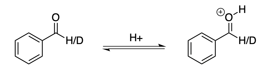
One interesting question that I’m revisiting is the following: when protonating benzaldehyde, what is the H/D equilibrium isotope effect at the aldehyde proton? This question was relevant for the H/D KIE experiments we conducted in our study of the asymmetric Prins cyclization. (The paper hasn’t gotten much attention, but it’s probably the most “classic” organic chemistry paper I’ve worked on, with a minimum of weird computational details or bizarre analytical techniques.)
Since the H/D bond isn’t involved in the reaction, we won’t see a primary effect; so we know we have to be thinking in terms of secondary effects. The most common reason to observe a secondary isotope effect is changes in hybridization: sp3 to sp2 gives a normal effect, whereas sp2 to sp3 gives an inverse effect. From this perspective, it looks like the effect should be unity, since the carbon in question is sp2 in both structures.
Reality, however, disagrees. Hall and Milosevich report a EIE of 0.94 for benzaldehyde in aq. sulfuric acid, and Gajewski and co-authors compute an EIE of 0.83 for acetaldehyde at the MP2/6-31G(d,p) level of theory. I performed my own calculations at the M06-2X/jun-cc-pVTZ level of theory and obtained an EIE of 0.851 with PyQuiver, qualitatively consistent with the above results.
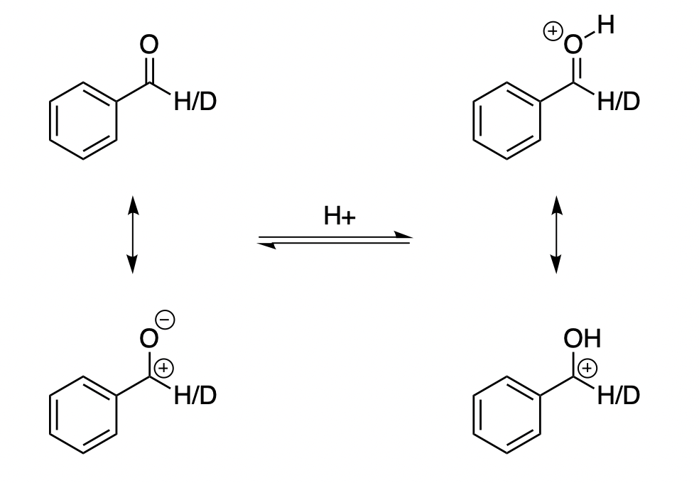
Where does this EIE come from? It’s helpful to think of benzaldehyde as possessing multiple resonance forms:
We typically think of the neutral resonance form on the top left, but you can also imagine putting a positive charge on carbon and a negative charge on oxygen to create a zwitterion with a C–O single bond (bottom left). In neutral benzaldehyde, this resonance form is substantially disfavored, but in protonated benzaldehyde it doesn’t look any worse than the “normal” top resonance form!
If this is true, we’d expect the C–O bond order to decrease from 2 in neutral benzaldehyde to ~1.5 in protonated benzaldehyde. Indeed, in my calculations the bond length increases from 1.20 Å to 1.28 Å upon protonation—so it seems the double bond character is decreasing! It’s not quite the same as going from sp2 to sp3, but the inverse KIE begins to make sense.
(This is purely guesswork, but my guess would be that the differences between the two structures are attenuated in a polar solvent like water. The zwitterionic resonance form of the neutral structure will be stabilized and thus the neutral aldehyde will be more polar, making the change to the oxocarbenium less drastic. This might explain why the measured EIE in water is smaller—although this might also be due to counterion effects, or something completely unrelated.)
Let’s go a level deeper. According to Streitwieser, secondary KIEs associated with hyperconjugation originate from the creation or destruction of the c. 800 cm-1 out-of-plane bending vibrations of Csp2–H hydrogens, which are markedly lower in frequency than the c. 1350 cm-1 bending vibrations associated with Csp3–H hydrogens.
Raising the frequency of a mode increases the energy required to inhabit the ground vibrational state (the “zero-point energy”)—but deuterium is heavier and vibrates more slowly, meaning that it possesses less ZPE and is less affected by these changes. So when an 800 cm-1 sp2 mode transforms to a 1350 cm-1 sp3 mode, the ZPE increases, but less for D than for H, so D is favored. Conversely, when a 1350 cm-1 sp3 mode transforms to a 800 cm-1 sp2 mode, the ZPE decreases, but less for D than for H, so H is favored. (For a more complete explanation, see this presentation by Rob Knowles.)
This effect is complicated for benzaldehyde by the fact that the out-of-plane bend of the aldehyde couples to the out-of-plane bend of the phenyl ring, so there are several modes involving out-of-plane vibration of the aldehyde proton. When I compared the out-of-plane bend of the aldehyde H in both structures, I saw only minimal differences: 771, 963, 1040, and 1051 cm-1 for the neutral species, as compared to 790, 1003, and 1061 cm-1 for the protonated species. These small differences can’t be responsible for the observed effect.
In contrast, the in-plane C–H bend shows a big change—1430 cm-1 for benzaldehyde, but 1644 cm-1 for the oxocarbenium (it seems to couple to the C–O stretch; the reduced mass increases from 1.26 amu to 3.52 amu). Applying Streitweiser’s formula for estimating the isotope effect for a specific mode gives a pretty good match:
I don’t understand this area well enough to comment on why there’s a change in the in-plane vibrational frequency and not the out-of-plane vibrational frequency, nor do I understand how to deconvolute the effects of mode-to-mode coupling. Nevertheless, this provides a tentative physical rationale for the observation.
On a more abstract level, this case study illustrates why isotope effects are such a good tool. Any transformation that perturbs the vibrational frequencies of a given molecule can, in principle, be monitored by isotope effects without affecting the electronic energy surface at all. So, although the precise nature and magnitude of the effect might be hard to predict a priori, it’s not surprising that a transformation as dramatic as protonating a functional group produces a sizable isotope effect.