In many applications, including cheminformatics, it’s common to have datasets that have too many dimensions to analyze conveniently. For instance, chemical fingerprints are typically 2048-length binary vectors, meaning that “chemical space” as encoded by fingerprints is 2048-dimensional.
To more easily handle these complex datasets (and to bypass the “curse of dimensionality”), it’s common practice to use a dimensionality reduction algorithm to convert the data to a low-dimensional space. In this post I want to compare and contrast three approaches to dimensionality reduction, and discuss the challenges with low-dimensional embeddings in general.
There are many approaches to dimensionality reduction, but I’m only going to talk about three here: PCA, tSNE, and UMAP.
Principal component analysis (PCA) is perhaps the most famous dimensionality reduction algorithm, and is commonly used in a variety of scientific fields. PCA works by transforming the data into a new set of coordinates such that the first coordinate vector explains the largest amount of the variance, the second coordinate vector the next most variance, and so on and so forth. It’s pretty common for the first 5–20 dimensions to capture >99% of the variance, meaning that the subsequent dimensions can essentially be discarded wholesale.
tSNE (t-distributed stochastic neighbor embedding) and UMAP (uniform manifold approximation and projection) are alternative dimensionality reduction approaches, based on much more complex algorithms. To quote Wikipedia:
The t-SNE algorithm comprises two main stages. First, t-SNE constructs a probability distribution over pairs of high-dimensional objects in such a way that similar objects are assigned a higher probability while dissimilar points are assigned a lower probability. Second, t-SNE defines a similar probability distribution over the points in the low-dimensional map, and it minimizes the Kullback–Leibler divergence (KL divergence) between the two distributions with respect to the locations of the points in the map.
UMAP, at a high level, works in a very similar way, but uses some fancy topology to construct a “fuzzy simplicial complex” representation of the data in high-dimensional space, and then projects this representation down into a lower dimension (more detailed explanation). Practically, UMAP is a lot faster than tSNE, and is becoming the algorithm of choice for most cheminformatics applications. (Although, in fairness, there are ways to make tSNE faster.)
For the purposes of this post, I chose to study Abbie Doyle’s set of 2683 aryl bromides (obtained from Reaxys, with various filters applied). I used the RDKIT7 fingerprint to generate a 2048-bit encoding of each aryl bromide, computed a distance matrix using Tanimoto/Jaccard distance, and then used each dimensionality reduction technique to generate a 2-dimensional embedding.
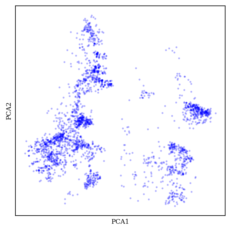
Let’s look at PCA first:
PCA generally creates fuzzy-looking blobs, which sometimes show some amount of meaningful structure but don’t really display many sharp boundaries.
Now, let’s compare to tSNE:
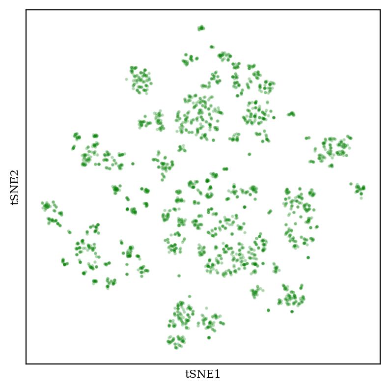
tSNE creates “blob-of-blob” plots which show many tight clusters arranged together in some sort of vague pattern. The size and position of the clusters can be tuned by changing the “perplexity” hyperparameter (see this StackOverflow post for more discussion, and this excellent post for demonstrations of how tSNE can be misleading).
What about UMAP?
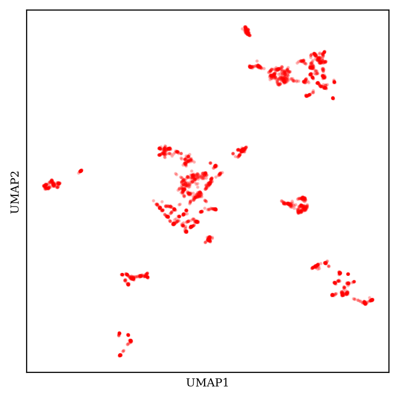
UMAP also creates tight tSNE-like clusters, but UMAP plots generally have a much more variable overall shape—the clusters themselves are tighter and scattered across more space. (These considerations are complicated by the fact that UMAP has multiple tunable hyperparameters, meaning that the exact appearance of the plot is substantially up to the end user.)
The debate between tSNE and UMAP is spirited (e.g.), but for whatever reason people in chemistry almost exclusively use UMAP. (See, for instance, pretty much every paper I taked about in this post.)
An important thing that I’m not showing here, but which bears mentioning, is that the clusters in all three plots are actually chemically meaningful. For instance, each cluster in the tSNE plot generally corresponds to a different functional group: carboxylic acids, alkynes, etc. So the graphs do in some real sense correspond to the intuition we have about molecular similarity, which is good! (You can use molplotly to visualize these plots very easily.)
How well are distances from the high-dimensional space preserved in the 2D embedding? Obviously the distances won’t all be the same, but ideally the mapping would be monotonic: if distance A is greater than distance B in the high-dimensional space, we would like distance A to also be greater than distance B in the low-dimensional space.
We can measure this with Spearman correlation, which is like a Pearson correlation (AKA “r-squared”) but without the assumption of linearity. A Spearman correlation coefficient of 1 indicates a perfect monotonic relationship, while a coefficient of 0 indicates no relationship. Let’s plot the pairwise distances from each embedding against the true distances and compare the Spearman coefficients:
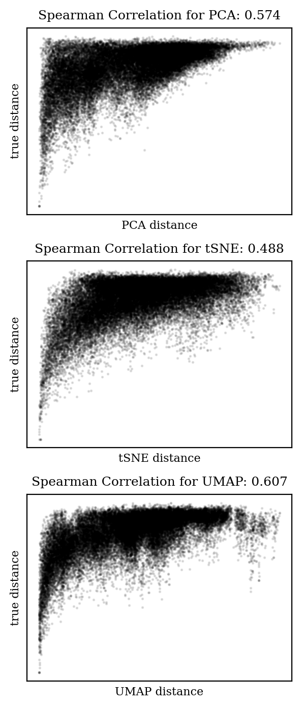
In each case, the trend is in the right direction (i.e. increased distance in high-dimensional space is correlated with increased distance in low-dimensional space), but the relationship is far from monotonic. It’s clear that there will be plenty of cases where two points will be close in low-dimensional space and far in high-dimensional space.
Does this mean that UMAP, tSNE, and PCA are all failing? To understand this better, let’s plot a histogram of all the distances in each space:
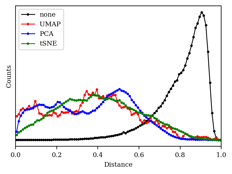
We can see that the 2048-dimensional space has a very distinct histogram. Most of the compounds are pretty different from one another, and—crucially—most of the distances are about the same (0.8 or so). In chemical terms, this means that most of the fingerprints share a few epitopes in common, but otherwise are substantially different, which is unsurprising since fingerprints in general are quite sparse.
Unfortunately, “lots of equidistant points” is an extremely tough pattern to recapitulate in a low-dimensional space. We can see why with a toy example: in 2D space, we can only have 3 equidistant points (an equilateral triangle), and in 3D space, we can only have 4 equidistant points (a tetrahedron). More generally, if we want N equidistant points, we need to be in RN-1 (N-1 dimensional Euclidean space). We can relax this requirement a little bit if we’re willing to accept approximate equidistance, but the general principle still holds: it’s hard to recapitulate lots of equidistant points in a low-dimensional space.
As expected, then, we can see that the histogram of each of our algorithms looks very different from the ideal distance histogram.
Both tSNE and UMAP take the nearest neighbors of each point explicitly into account, and claim to preserve the local structure of the points as much as possible. To put these claims to the test, I looked at the closest 30 neighbors of each point in high-dimensional space, and then checked how many of those neighbors made it into the closest 30 neighbors in low-dimensional space.
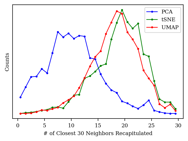
We can see that PCA only preserves about 30–40% of each point’s neighbors, whereas PCA and UMAP generally preserve 60% of the neighbors: not perfect, but much better.
I chose to look at 30 neighbors somewhat arbitrarily: what happens if we change this number?
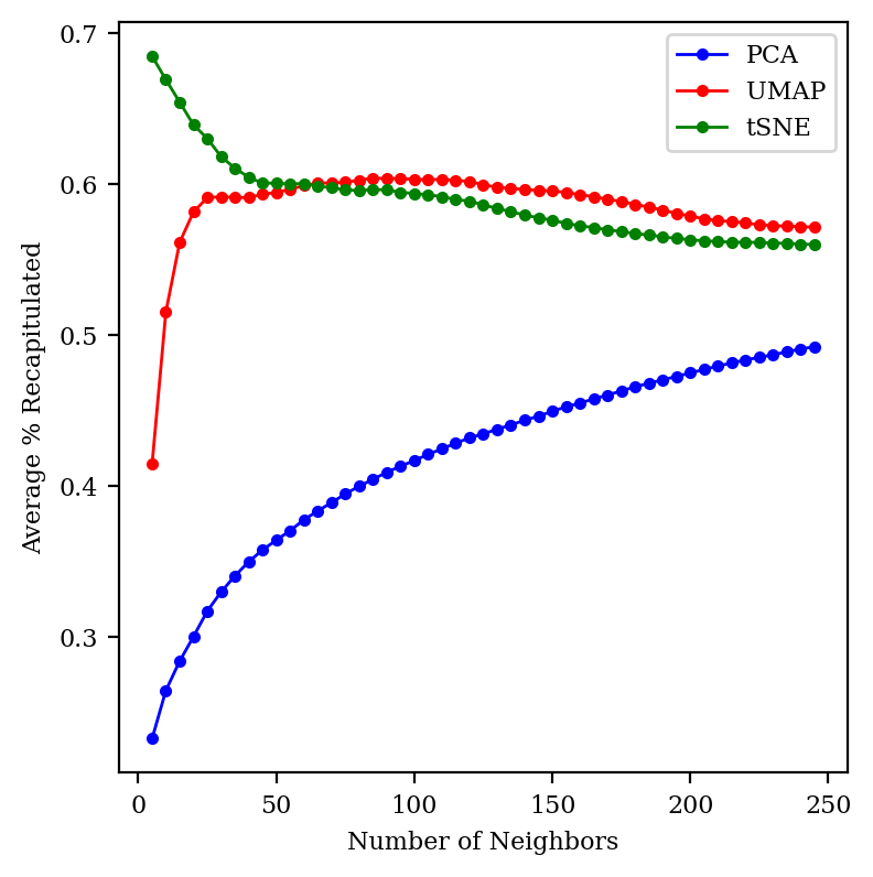
We can see that UMAP and tSNE both preserve about 60% of the neighbors across a wide range of neighborhood sizes, while PCA gets better as we zoom out more. (At the limit where we consider all 2683 points as neighbors, every method will trivially achieve perfect accuracy.) tSNE does much better than UMAP for small neighborhoods; I’m not sure why!
Another way to think about this is in terms of the precision–recall tradeoff. In classification, “precision” refers to a classifier’s ability to avoid false positives, while “recall” refers to a classifier’s ability to avoid false negatives. What does this mean in the context of embedding?
Imagine looking at all points in the neighborhood of our central point in high-dimensional space, and then comparing to the points within a certain radius of our point in low-dimensional space. As we increase the radius, we expect to see more of the correct neighbor points in low-dimensional space, but we also expect to see more “incorrect neighbors” that aren’t really there in the high-dimensional space. (This paper discusses these issues nicely, as does this presentation.)
So low radii lead to high precision (most of the points are really neighbors) but low recall (we’re not finding most of the neighbors), while high radii lead to low precision and high recall. We can thus study the performance of our embedding by graphing the precision–recall curve for various neighborhood sizes. The better the embedding, the closer the curve will come to the top right:
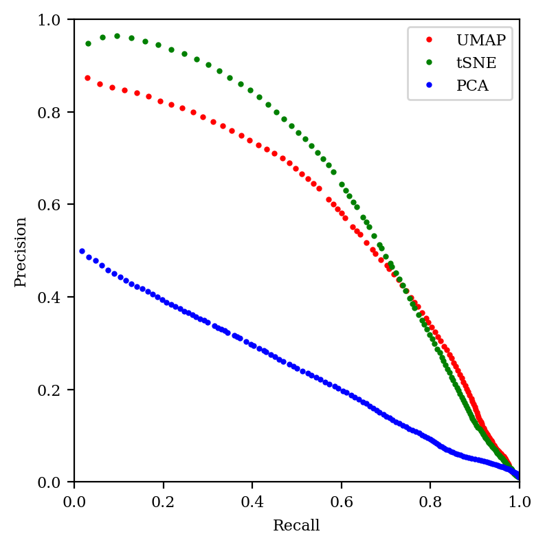
We can see that tSNE does better in the high precision/low recall area of the curve (as we saw in the previous graph), but otherwise tSNE and UMAP are quite comparable. In contrast, PCA is just abysmal.
The big conclusion of this section is that, if you’re doing something that depends on the local structure of the data, you should avoid PCA.
Since the root of our issues here is trying to represent a 2048-dimensional distance matrix in 2 dimensions, one might wonder if we could do better by expanding to 3, 4, or more dimensions. This would make visualization tricky, but might still be suitable for other operations (like clustering).
tSNE gets very, very slow in higher dimensions, so I focused on PCA and UMAP for this study. I started out by comparing the Spearman correlation for PCA and UMAP up to 20 dimensions:
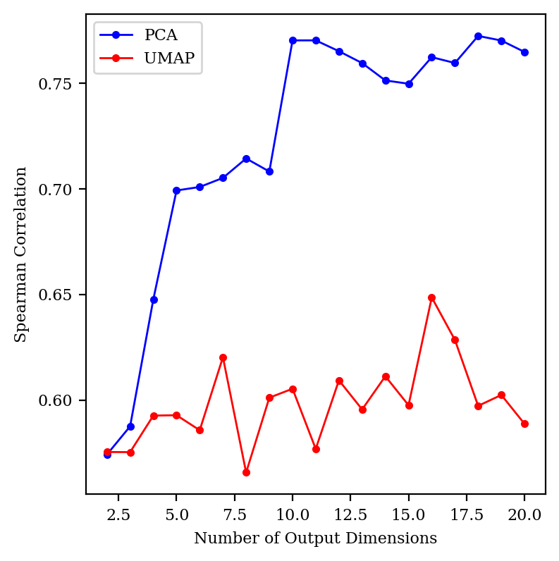
Surprisingly, UMAP doesn’t seem to get any better in high dimensions, but PCA does. (Changing the number of neighbors didn’t help UMAP at all.)
How do our other metrics look with high-dimensional PCA?
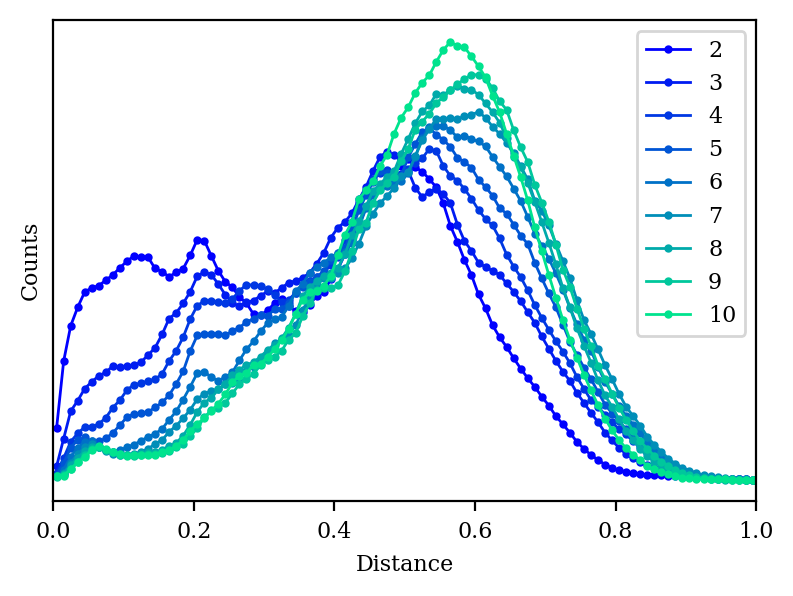
As we increase the number of dimensions, the distance histogram starts to approach the correct distribution.
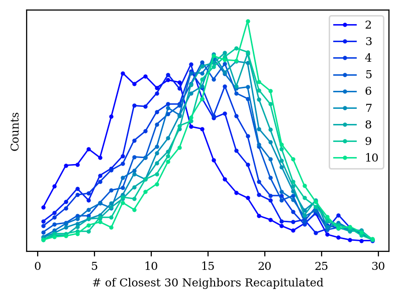
We also start to do a better job capturing the local structure of the graph, although we’re still not as good as tSNE or UMAP even at 10 dimensions.
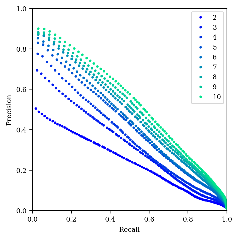
And our precision–recall graph is still pretty dismal when compared to tSNE or UMAP. So, it seems like if distances are what matters, then high-dimensional PCA is an appealing choice—but if local structure is what matters, tSNE or UMAP is still superior.
My big takeaway from all of this is: dimensionality reduction is a lossy process, and one where you always have to make tradeoffs. You’re fundamentally throwing away information, and that always has a cost: there’s no such thing as a free lunch. As such, if you don’t have to perform dimensionality reduction, then my inclination would be to avoid it. (People in single-cell genomics seem to have come to a similar conclusion.)
If you really need your data to be in a low-dimensional space (e.g. for plotting), then keep in mind what you’re trying to study! PCA seems to do a slightly better job with distances (although I’m sure there are more sophisticated strategies for distance-preserving dimensionality reduction), while tSNE and UMAP seem to do much, much better with local structure.
Thanks to Michael Tartre for helpful conversations, and the students in Carnegie Mellon’s “Digital Molecular Design Studio” class for their thought-provoking questions on these topics.